Beyond CPU - Hardware Acceleration for Edge AI

Hardware Acceleration with MemryX MX3 on Raspberry Pi 5.

Introduction

Throughout this course, we’ve explored various approaches to deploying AI models at the edge. We started with TensorFlow Lite running on the Raspberry Pi’s CPU, then moved to YOLO and ExecuTorch with optimized backends like XNNPACK. While these software optimizations significantly improve performance, they still rely on the general-purpose CPU to execute neural network operations.

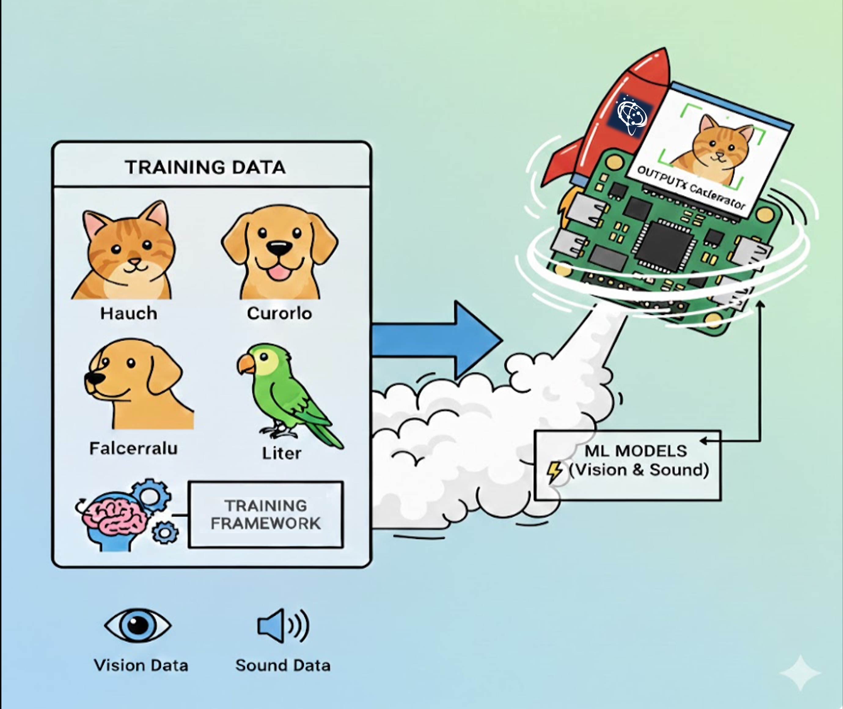
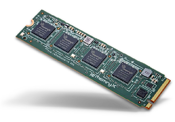
In this chapter, we’ll take the next step: dedicated hardware acceleration. We’ll use the MemryX MX3 M.2 AI Accelerator Module—a specialized processor designed specifically for neural network inference. The MX3 module contains four AI accelerator chips that can run deep learning models with dramatically lower latency and power consumption compared to CPU execution.

Why Hardware Acceleration?

Consider the requirements for real-time edge AI applications: - Latency: Autonomous systems need predictions in milliseconds - Power efficiency: Battery-powered devices must conserve energy - Throughput: Multi-camera systems may need to process several streams simultaneously - Cost: System designs often cannot afford high-end GPUs

The MX3 addresses these challenges with a unique architecture: - At-memory computing: All memory is integrated on the accelerator, eliminating bandwidth bottlenecks - Pipelined dataflow: Optimized for streaming inputs with a batch size of 1 - Floating-point accuracy: No quantization required (though supported) - Low power: Maximum 10W for four accelerator chips

For learning more about AI Acceleration, please refer to MLSys book and how the MemryX module works, read the Architecture Overview.

Our goal

By the end of this lab, we will have installed and configured the MX3 hardware on a Raspberry Pi 5, set up the MemryX SDK and development environment, and gained a clear understanding of the MX3 compilation and deployment workflow. We will also compile neural network models for execution on the MX3 accelerator, compare their performance against CPU-based inference while analyzing the trade-offs, and finally build a complete end-to-end inference pipeline using the MemryX Python API.

Hardware Installation and Verification

Prerequisites

Before starting this lab, we should have:

Raspberry Pi 5 with M.2 HAT+ adapter (or similar)

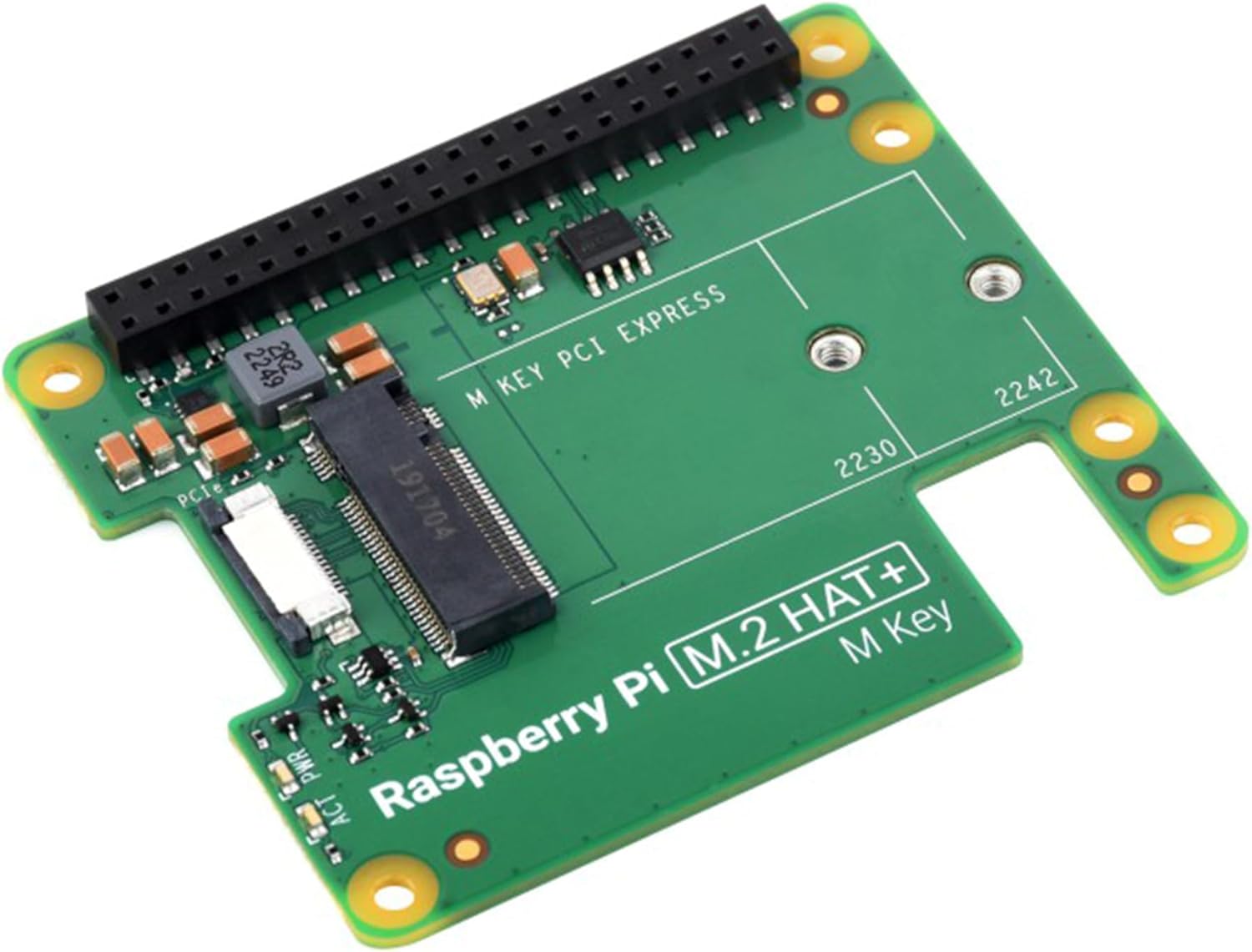
IMPORTANT NOTE: MemryX recommends the GeeekPi N04 M.2 2280 HAT as an excellent choice for the Raspberry Pi 5. It delivers solid power and fits the 2280 MX3 M.2 form factor. Some hats can lead to instabilities, mainly due to PCIe speed (Gen3). The Raspberry Pi 5 can have stability issues on Gen3.

The Raspberry Pi M.2 HAT+ is a good option. It works very well, despite the fact that we should adapt the MX3 board to it (The MX3 is longer than the hat).

MemryX MX3 M.2 module with the heatsink installed

For heatsink installation, follow the video instructions: https://youtu.be/wNmka0nrRRE

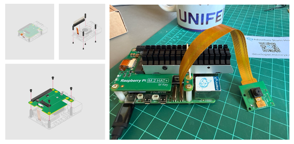
Installation and Cooling Considerations

It is essential to ensure we have sufficient cooling for the MemryX MX3 M.2 module, or we may experience thermal throttling and reduced performance. The chips will throttle their performance if they hit 100 °C.

During normal operation, the current MemryX MX3 temperature and throttle status can be viewed at any time with:

cat /sys/memx0/temperature

Or measurd continuay every 1 second, for example with the command:

watch -n 1 cat /sys/memx0/temperature

Verification

After installing the hardware, turn on the Raspberry Pi and verify the system setup.

ls /dev/memx*

It should return: /dev/memx0

If the device is not detected, see the Troubleshooting section below.

Let’s also check the initial temperature:

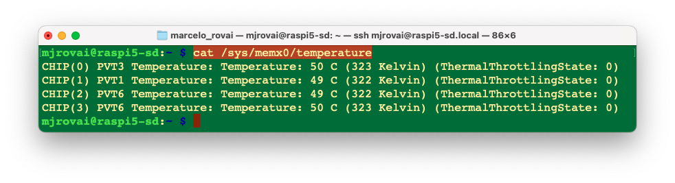
The lab temperature at the time of the above measurement was 25 °C.

Software Installation

Create Project Directory

First, we should create a project directory:

cd Documents
mkdir MEMRYX
cd MEMRYX

Python Version Management with Pyenv

Verify your Python version:

python --version

If using the latest Raspberry Pi OS (based on Debian Trixie), it should be:

Python 3.13.5

Or, if the OS is the Legacy version:

Python 3.11.2

Important: As of January 2026, MemryX officially supports only Python 3.09 to 3.12. Python 3.13.5 is too new and will likely cause compatibility issues. Since Debian Trixie ships with Python 3.13 by default, we’ll need to install a compatible Python version alongside it.

One solution is to install Pyenv, which allows us to easily manage multiple Python versions for different projects without affecting the system Python.

If the Raspberry Pi OS is the legacy version, the Python version should be 3.11, and it is not necessary to install Pyenv.

Installing Pyenv on Debian Trixie

If you need to install Pyenv on Debian Trixie, follow these steps:

# Install dependencies
sudo apt install -y make build-essential libssl-dev zlib1g-dev \
libbz2-dev libreadline-dev libsqlite3-dev wget curl llvm \
libncursesw5-dev xz-utils tk-dev libxml2-dev libxmlsec1-dev \
libffi-dev liblzma-dev

# Install pyenv
curl https://pyenv.run | bash

# Add to ~/.bashrc
echo 'export PYENV_ROOT="$HOME/.pyenv"' >> ~/.bashrc
echo 'command -v pyenv >/dev/null || export PATH="$PYENV_ROOT/bin:$PATH"' \
>> ~/.bashrc
echo 'eval "$(pyenv init -)"' >> ~/.bashrc

# Reload shell
source ~/.bashrc

# Install Python 3.11.14
pyenv install 3.11.14

This process takes several minutes as it compiles Python from source.

Set Python Version for Project

Once Pyenv and the selected Python version are installed, define it for the project directory:

pyenv local 3.11.14

Checking the Python version again, we should see: Python 3.11.14.

MemryX Drivers and SDK Installation

The MemryX software stack consists of two main components:

Drivers (memx-drivers): Kernel-level drivers for PCIe communication with the accelerator hardware
SDK (memx-accl): Python libraries, neural compiler, runtime, and benchmarking tools

Prepare the System

Install the Linux kernel headers required for driver compilation:

sudo apt install linux-headers-$(uname -r)

Add MemryX Repository and Key

This command downloads the repository’s GPG key for package verification and adds the MemryX package repository:

wget -qO- https://developer.memryx.com/deb/memryx.asc | \
sudo tee /etc/apt/trusted.gpg.d/memryx.asc >/dev/null

echo 'deb https://developer.memryx.com/deb stable main' | \
sudo tee /etc/apt/sources.list.d/memryx.list >/dev/null

Update and Install Drivers and SDK

sudo apt update
sudo apt install memx-drivers memx-accl

Configure Platform Settings

Run the ARM setup utility to configure platform-specific settings. This opens a menu to select the platform and apply the necessary configurations (e.g., enabling PCIe Gen 3.0 on the Raspberry Pi 5):

sudo mx_arm_setup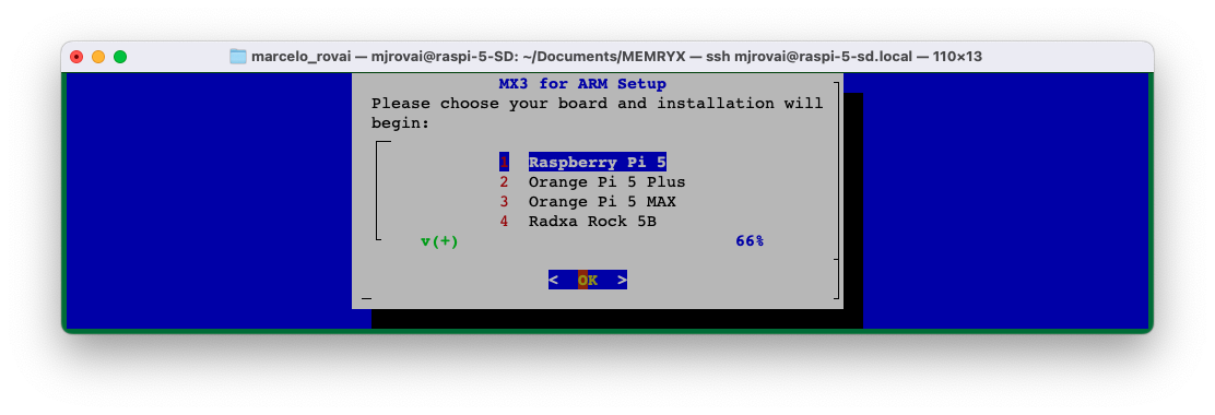

Select the appropriate option for your hardware, and press <OK> in the next page:

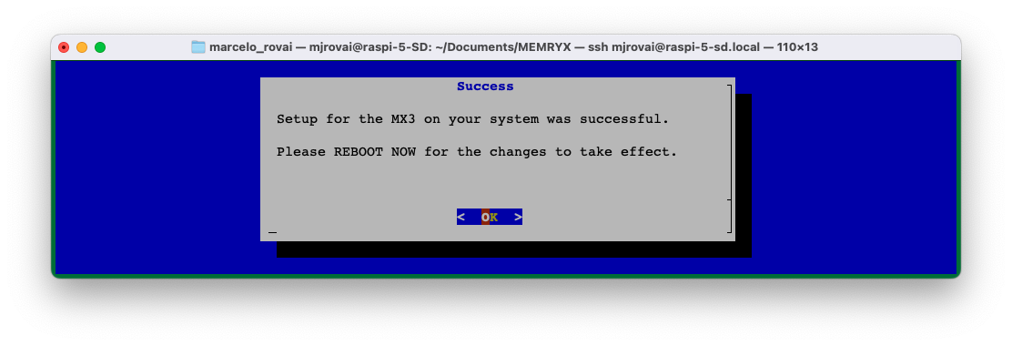
After configuration, reboot the system:

sudo reboot

Verify Driver Installation

After rebooting, verify that the MemryX driver is installed by checking its version:

apt policy memx-drivers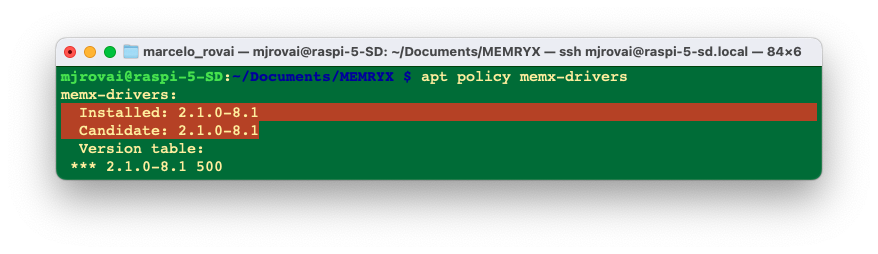

Install Utilities

Install additional utilities including GUI tools and plugins:

sudo apt install memx-accl-plugins memx-utils-gui

Prepare System Dependencies

Install system libraries required for the Python SDK:

sudo apt update
sudo apt install libhdf5-dev python3-dev cmake python3-venv build-essential

Install Tools (Inside Virtual Environment)

It’s best practice to use a virtual environment to avoid conflicts with system packages.

Create and activate a virtual environment:

python -m venv mx-env
source mx-env/bin/activate

Inside the environment, install the MemryX Python package:

pip3 install --upgrade pip wheel
pip3 install --extra-index-url https://developer.memryx.com/pip memryx

Verify the neural compiler is installed:

mx_nc --version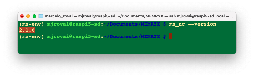

Verification

Verify the complete installation by running the built-in “hello world” benchmark:

mx_bench --hello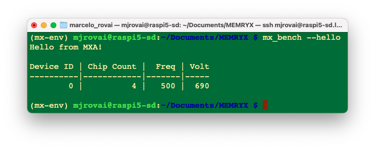

With the benchmark results, our MemryX MX3 is properly installed and ready to use.

Our First Accelerated Model

Understanding the MX3 Workflow

Working with the MemryX MX3 follows a straightforward four-step workflow that differs from traditional CPU-based inference:

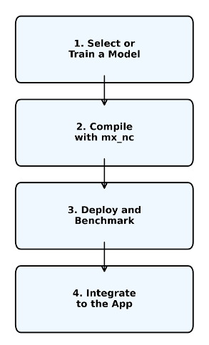
Step 1: Select or Train a Model

Start with a pre-trained model or train your own. MemryX supports models from major frameworks:

TensorFlow/Keras (.h5, SavedModel)
ONNX (.onnx)
PyTorch (.pt, .pth) (Should be converted to ONNX first)
TensorFlow Lite (.tflite)

The model remains in its original format—no framework-specific conversions needed yet. For this lab, we’re using MobileNetV2 from Keras Applications, but we could equally use a custom model we have trained for a specific task, as we have seen before.

Supported Operations: The MX3 supports most common deep learning operators (convolutions, pooling, activations, etc.). Check the supported operators if using custom architectures. Unsupported operations will fall back to CPU, though this is rare for standard vision models.

Step 2: Compile with Neural Compiler

The MemryX Neural Compiler (mx_nc) transforms the model into a DFP (Dataflow Package):

mx_nc [options] -m <model_file>

The MemryX Neural Compiler, mx_nc, is a command‑line tool that takes one or more neural‑network models (Keras, TensorFlow, TFLite, ONNX, etc.) and compiles them into a MemryX Dataflow Program (DFP) that can run on MemryX accelerators (MXA). Internally, it does framework import, graph optimization (fusion/splitting, operator expansion, activation approximation), resource mapping on the MXA cores, and finally emits the DFP used by the runtime or simulator.

What mx_nc does:

Compiles models into a single DFP file per compilation, then loads it onto one or more MXA chips to run inference.
Supports multi‑model, multi‑stream, and multi‑chip mapping, automatically distributing models and layers across available MX3 devices for higher throughput.
Handles mixed‑precision weights (per‑channel 4/8/16‑bit) while keeping activations in floating point on the accelerator. By default, MemryX quantizes weights to INT8 precision and activations to BFloat16.
Can crop pre/post‑processing parts of the graph so the MXA focuses on the core CNN/ML operators while the host CPU runs the cropped sections.

What happens during compilation?

Model parsing: Loads the model and extracts the computational graph
Graph optimization: Fuses operations, eliminates redundancies
Operator mapping: Maps each layer to MX3 hardware instructions
Dataflow scheduling: Determines optimal execution order for pipelined processing
Memory allocation: Assigns on-chip memory for all intermediate activations
Multi-chip distribution: If using multiple chips, partitions the workload

The compiler is surprisingly tolerant—most models compile without any modifications. If a layer isn’t supported, you’ll get a clear error message indicating which operation failed.

Key command‑line options (high level)

Model specification:
- -m / --models – input model file(s) (e.g. .h5, .pb, .onnx, TFLite).
- Multi‑model example: mx_nc -v -m model_0.h5 model_1.onnx.
Input shapes:
- -is, --input_shapes – specify input shape(s) when they cannot be inferred, always in NHWC order (e.g. "224,224,3").
- Supports "auto" for models where shapes can be inferred: -is "auto" "300,300,3".
Cropping / pre‑ and post‑processing control:
- --autocrop – experimental automatic cropping of pre/post‑processing layers. See the YOLOv8 example further in this chapter.
- --inputs, --outputs – manually set which graph nodes are treated as the MXA inputs/outputs; everything outside is cropped to run on the host.
- For multi‑model graphs, inputs/outputs of different models are separated with | (vertical bar).
- --model_in_out – JSON file describing model inputs/outputs for more complex single or multi‑model cases.
Multi‑chip / system sizing:
- -c – number of MXA chips; -c 2 means compile for two chips and distribute workload across them.
Diagnostics / verbosity:
- -v, -vv, etc. – increase verbosity, useful to inspect graph transformations and cropping decisions.
Extensions / unsupported patterns:
- --extensions – load Neural Compiler Extensions (.nce files or builtin names) to add or patch graph handling (e.g., complex transformer subgraphs or unsupported ops) without a new SDK release.

For the complete option list (including less common flags), run mx_nc -h or consult the Neural Compiler page in the MemryX Developer Hub, which documents all arguments and includes usage examples for single‑model, multi‑model, cropping, and mixed‑precision flows.

Compilation time varies by model complexity:

Small models (MobileNet): ~30 seconds
Medium models (ResNet50): ~2 minutes
Large models (EfficientNet): ~5 minutes

Once compiled, the DFP file is portable across all MX3 hardware.

Step 3: Deploy and Benchmark

Before integrating into our application, we can verify performance with the benchmarking tool:

mx_bench -d <dfp_file> -f <num_frames>

The benchmarker: - Generates synthetic input data matching the model’s input shape - Runs warm-up inferences to stabilize performance - Measures throughput (FPS), latency, and chip utilization - Reports first-inference latency (includes loading overhead)

Why benchmark separately? Real-world applications involve preprocessing (image loading and resizing) and postprocessing (parsing outputs). Benchmarking isolates pure inference performance, letting to identify bottlenecks in our full pipeline.

Step 4: Integrate into the Application

Finally, integrate the accelerator into our Python application using the MemryX API:

from memryx import SyncAccl  # or AsyncAccl for concurrent processing

# Initialize accelerator with our DFP
accl = SyncAccl(dfp="model.dfp")

# Run inference
output = accl.run(input_data)

# Process results
# ...

# Clean up
accl.shutdown()

Synchronous vs. Asynchronous APIs:

SyncAccl: Blocking calls, simple to use, good for single-stream processing
AsyncAccl: Non-blocking, better for multi-stream or real-time applications

The API handles all hardware communication, memory transfers, and scheduling. Our code just provides input tensors and receives output tensors—the complexity is abstracted away.

Complete Workflow Example

Let’s see the four steps in action with MobileNetV2:

# Step 1: Get a model (already trained)
python3 -c "import tensorflow as tf; \
tf.keras.applications.MobileNetV2().save('mobilenet_v2.h5');"

# Step 2: Compile to DFP
mx_nc -v -m mobilenet_v2.h5

# Step 3: Benchmark
mx_bench -d mobilenet_v2.dfp -f 1000

# Step 4: Integrate (see full Python script in next section)
python run_inference_mobilenetv2.py

This workflow is remarkably consistent across models and use cases. Once we’ve done it for one model, adapting to others is straightforward.

Key Takeaway: The MX3 workflow separates compilation (done once) from inference (done repeatedly). This “compile-once, run-many” approach means the optimization overhead is amortized over thousands or millions of inferences in production.

Download and Compile MobileNetV2

In Keras Applications, we can find deep learning models that are provided with pre-trained weights. These models can be used for prediction, feature extraction, and fine-tuning.

Let’s download MobileNetV2, which was used in previous labs:

python3 -c "import tensorflow as tf; \ 
tf.keras.applications.MobileNetV2().save('mobilenet_v2.h5');"

The model is saved in the current directory as mobilenet_v2.h5.

Next, we will compile the MobileNetV2 model using the MemryX Neural Compiler. This step verifies that both the compiler and the SDK tools are installed and functioning as expected:

mx_nc -v -m mobilenet_v2.h5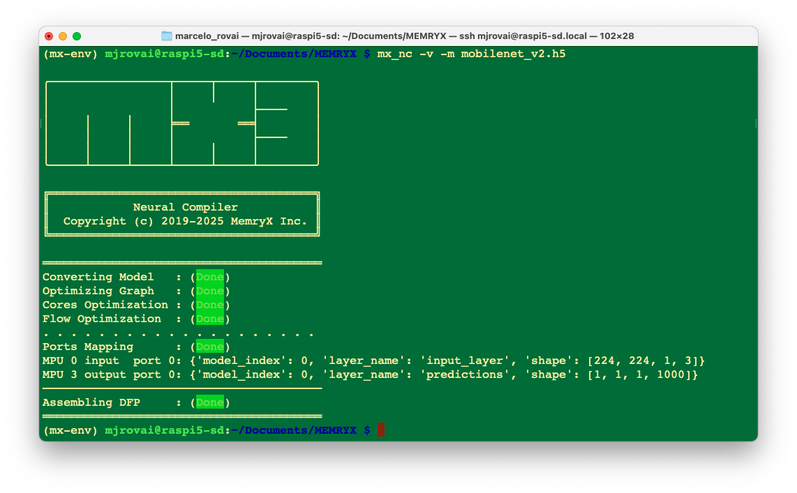

The compiled model, mobilenet_v2.dfp, is saved in the current folder.

What is a DFP file?

The .dfp (Dataflow Package) file is MemryX’s proprietary compiled format. Unlike standard model formats (H5, ONNX, etc.) that describe the network architecture, a DFP file contains:

Optimized operator graph: The network restructured for dataflow execution
Memory layout: Pre-calculated memory allocations for at-memory computing
Chip mappings: Instructions for distributing work across the four MX3 accelerators
Quantization parameters: If applicable, the bit-width and scaling factors

The neural compiler (mx_nc) performs this transformation automatically, with no manual tuning required. The compilation process: 1. Parses the input model (H5, ONNX, TFLite, etc.) 2. Maps operators to MX3-supported operations 3. Optimizes the dataflow graph 4. Allocates memory on-chip 5. Generates the DFP binary

This is why compilation takes a few minutes, but inference is blazingly fast—all the optimization work happens once, upfront.

Benchmarking Performance

Now that the model is compiled, it’s time to deploy it and run a benchmark to test its performance on the MXA hardware. We will run 1000 frames of random data through the accelerator to measure performance metrics:

mx_bench -v -d mobilenet_v2.dfp -f 1000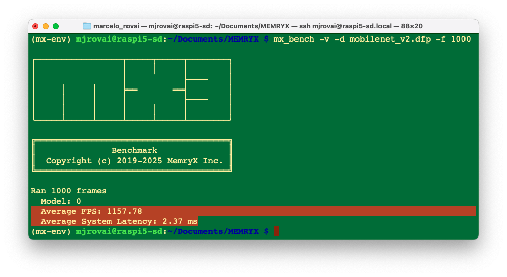

Let’s understand what these metrics mean:

FPS (Frames Per Second): How many images the accelerator can process per second (~1,200 FPS for MobileNetV2)
Latency: Time for a single inference (shown as “Avg” in the output)
- Subsequent inferences: True steady-state performance (~2ms)
Throughput: Total data processed per second

The benchmark runs with random input data, which is why we see consistent performance. Real-world performance with actual images should be similar once the preprocessing pipeline is optimized, but we have found bigger latency.

In true dataflow architecture, latency and FPS are not coupled in the traditional sense; latency does not equal 1/FPS. Note that even though latency is ~2ms in the above benchmarking results, FPS is not measured to be 1000 ms / 2 ms = 500 FPS; rather, the FPS from the benchmarking results is ~1160.

In MemryX’s dataflow architecture, the “usual” rule (latency = 1/FPS) only applies to frame‑to‑frame latency, not to end‑to‑end in‑to‑out latency for a single frame. That is why we see ~2 ms latency per frame, yet still measure around 1160 FPS in MX3 benchmarks.

Two different latencies MemryX explicitly distinguishes two metrics.

Latency 1 (frame‑to‑frame latency): Time between consecutive outputs once the pipeline is full. Its reciprocal is FPS.
Latency 2 (full in‑to‑out latency): Time from when the first input frame enters the system (host + MX3 pipeline) until its output appears. This can be larger, but it does not set the FPS.

In a streaming, pipelined accelerator like MX3, multiple frames are in‑flight simultaneously, so the pipeline “fills” once and then produces results at a steady cadence.

Building an Inference Application

Now let’s build a complete inference application that processes real images and compares CPU vs. MX3 performance.

Prepare Directory Structure

Let’s create subdirectories for organization:

mkdir models
mkdir images

Download Test Image

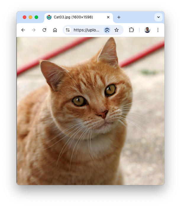
Load an image from the internet, for example, a cat (for comparison, it is the same as used on previous chapters):

wget "https://upload.wikimedia.org/wikipedia/commons/3/3a/Cat03.jpg" \
     -O ./images/cat.jpg

Here is the image:

Understanding Input Requirements

All neural networks expect input data in a specific format, determined during training. For MobileNetV2 trained on ImageNet:

Input shape: (224, 224, 3) - RGB images at 224x224 pixels
Batch dimension: Models expect batch inputs, so (1, 224, 224, 3) for single images
Preprocessing: MobileNetV2 uses specific normalization (scaling pixel values to [-1, 1])
Color channels: RGB order (not BGR)

The preprocessing must match exactly what was used during training, or accuracy will suffer.

Getting the Labels

For inference, we will need the ImageNet labels. The following function checks if the file exists, and if not, downloads it:

import os, json
from pathlib import Path
import requests

MODELS_DIR = Path("./models")
IMAGENET_JSON = MODELS_DIR / "imagenet_class_index.json"
IMAGENET_JSON_URL = (
    "https://storage.googleapis.com/download.tensorflow.org/data/\
    imagenet_class_index.json"
)

# ---- one-time label download ----
def ensure_imagenet_labels():
    MODELS_DIR.mkdir(parents=True, exist_ok=True)
    if IMAGENET_JSON.exists():
        return
    print("Downloading ImageNet class index...")
    resp = requests.get(IMAGENET_JSON_URL, timeout=30)
    resp.raise_for_status()
    IMAGENET_JSON.write_bytes(resp.content)
    print("Saved:", IMAGENET_JSON)

The function load_idx2label() loads the labels into a list:

def load_idx2label():
    with open(IMAGENET_JSON, "r") as f:
        class_idx = json.load(f)
    idx2label = [class_idx[str(k)][1] for k in range(len(class_idx))]
    return idx2label

Image Preprocessing

The image used for inference should be preprocessed in the same way as during model training. keras.applications.mobilenet_v2.preprocess_input() takes an image of shape (224, 224) and converts it to (1, 224, 224, 3):

import numpy as np
from PIL import Image
import tensorflow as tf
from tensorflow import keras

def load_and_preprocess_image(image_path):
    img = Image.open(image_path).convert("RGB").resize((224, 224))
    arr = np.array(img).astype(np.float32)
    arr = keras.applications.mobilenet_v2.preprocess_input(arr)
    arr = np.expand_dims(arr, 0)  # Add batch dimension
    return arr

Prepare Input Tensor

The processed image will serve as the model’s input tensor (x):

ensure_imagenet_labels()
idx2label_full = load_idx2label()  # length 1000 for ImageNet

IMAGE_PATH = Path("./images/cat.jpg")
x = load_and_preprocess_image(IMAGE_PATH)

Run Inference on MemryX Accelerator (MXA)

Move the models (the original and compiled) to the models folder and set up the paths:

MODELS_DIR = Path("./models")
DFP_PATH = MODELS_DIR / "mobilenet_v2.dfp"
KERAS_PATH = MODELS_DIR / "mobilenet_v2.h5"

Run inference on the compiled model using the MemryX accelerator:

from memryx import SyncAccl

accl = SyncAccl(dfp=str(DFP_PATH))
mxa_outputs = accl.run(x)

We get a list/array of outputs. In this case, with a shape of (1, 1000) and a dtype of float32. This output should be normalized to a NumPy array:

mxa_outputs = np.array(mxa_outputs)
if mxa_outputs.ndim == 3:
    mxa_outputs = mxa_outputs[0]

Decode the MXA Results

Now, using helper functions to extract top-k predictions:

def topk_from_probs(probs, k=5):
    """
    probs: (1, num_classes) or (num_classes,)
    Returns [(index, prob)] sorted by prob desc.
    """
    probs = np.array(probs)
    if probs.ndim == 2:
        probs = probs[0]
    # If outputs are logits, uncomment this:
    # probs = tf.nn.softmax(probs).numpy()
    s = probs.sum()
    if s > 0:
        probs = probs / s
    idxs = np.argsort(probs)[::-1][:k]
    return [(int(i), float(probs[i])) for i in idxs]

def label_for(idx, idx2label):
    if idx2label is not None and idx < len(idx2label):
        return idx2label[idx]
    return f"class_{idx}"

We can decode and print the results:

mxa_top5 = topk_from_probs(mxa_outputs, k=5)
print("\nMXA top-5:")
for idx, prob in mxa_top5:
    name = label_for(idx, idx2label_full)
    print(f"  #{idx:4d}: {name:20s}  ({prob*100:.1f}%)")

Expected output:

MXA top-5:
  # 282: tiger_cat             (38.6%)
  # 281: tabby                 (18.3%)
  # 285: Egyptian_cat          (15.2%)
  # 287: lynx                  (3.9%)
  # 478: carton                (1.7%)

Comparing CPU vs. MXA Performance

We can also run the unconverted model (mobilenet_v2.h5) on the CPU, applying the code to the same input tensor:

cpu_model = keras.models.load_model(KERAS_PATH)
cpu_outputs = cpu_model.predict(x)

num_classes = cpu_outputs.shape[-1]
idx2label = idx2label_full if num_classes == len(idx2label_full) else None

cpu_top5 = topk_from_probs(cpu_outputs, k=5)
print("\nCPU top-5:")
for idx, prob in cpu_top5:
    name = label_for(idx, idx2label)
    print(f"  #{idx:4d}: {name:20s}  ({prob*100:.1f}%)")

Expected output:

CPU top-5:
  # 282: tiger_cat             (58.4%)
  # 285: Egyptian_cat          (12.9%)
  # 281: tabby                 (11.6%)
  # 287: lynx                  (3.4%)
  # 588: hamper                (1.3%)

Despite the probabilities not being identical, both models reach the same top prediction. The slight differences are due to numerical precision variations between CPU and accelerator implementations.

Measuring Latency

Let’s create a complete Python script (run_inference_mobilenetv2.py) that also measures and compares latency for both CPU and MXA.

Note: The following sections break down the complete inference script into logical components. The full working script is available separately and integrates all these pieces together.

To measure latency accurately, we’ll add timing code:

import time

# Warm-up run
_ = accl.run(x)

# Timed inference
start = time.time()
mxa_outputs = accl.run(x)
mxa_latency = time.time() - start

print(f"\nMXA latency: {mxa_latency*1000:.2f} ms")

Run the complete script run_inference_comp_mobilenetv2.py in the terminal:

python run_inference_comp_mobilenetv2.py

Expected results:

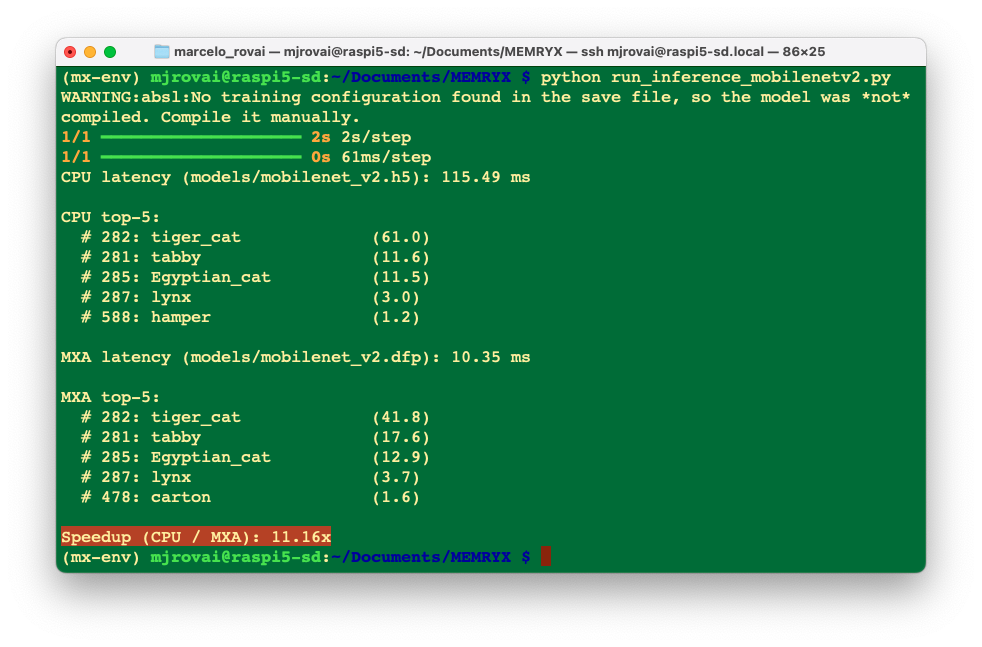
The Accelerator runs 11 times faster than the CPU!

The MobileNet V2 running with ExecuTorch/XNNPACK backend on a CPU has around 20 ms of latency.

Testing with Larger Models

We can also test a larger model like ResNet50:

# Download ResNet50
python3 -c "import tensorflow as tf; \
tf.keras.applications.ResNet50().save('resnet50.h5');"

# Compile
mx_nc -v -m resnet50.h5

# Run the script in the terminal:
python run_inference_comp_resnet50.py

The script can be found in the lab repo: run_inference_comp_resnet50.py in the terminal:

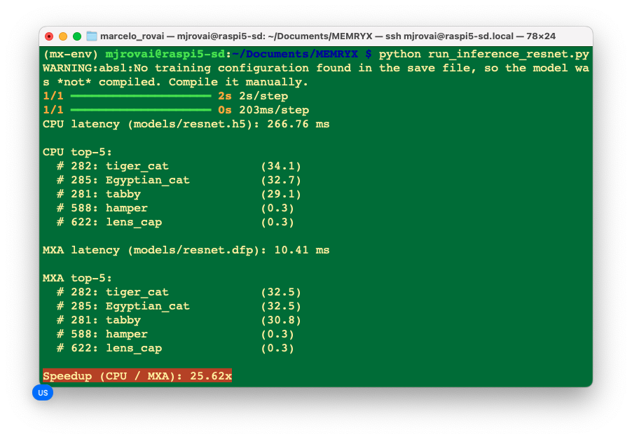
The performance improvements are even more dramatic with larger models!

Clean Shutdown

Always properly shut down the accelerator when done:

accl.shutdown()

BTW, to shut down the Raspberry Pi via SSH, we can use

sudo shutdown -h now

Folders Structure

Documents/MEMRYX/
├── run_inference_comp_mobilenetv2.py          # MobileNetV2 script
├── run_inference_comp_resnet50.py             # ResNet50 script
├── images/
│   ├── cat.jpg                           # Test image
├── models/
│   ├── mobilenet_v2.h5                   # Original model
│   ├── mobilenet_v2.dfp                  # Compiled model
│   ├── resnet50.h5                       # Original model
│   ├── resnet50.dfp                      # Compiled model
│   └── imagenet_class_index.json         # Labels (auto-downloaded)
└── mx-env/

Performance Comparison Summary

Here’s how the MX3 compares across different deployment approaches we’ve covered in this course:

Approach	Hardware	MobileNetV2 Latency	ResNet50 Latency	Power (Active)
TFLite (CPU)	Raspberry Pi 5	~110 ms	~266 ms	~
ExecuTorch/XNNPACK	Raspberry Pi 5	~20 ms	NA	~
MemryX MX3	Dedicated accelerator	~10 ms	~10 ms	~

Key Observations

25x faster than unoptimized TFLite on CPU (Resnet50)
2x faster than highly optimized ExecuTorch with XNNPACK (MobileNetV2)
Minimal CPU load: The host CPU is free for preprocessing, postprocessing, and application logic
Consistent latency: Hardware acceleration provides deterministic performance
Power efficiency: Not measured

When to Use the MX3?

The MemryX MX3 is ideal for:

✅ Real-time applications requiring <20ms latency
✅ Multi-stream processing (multiple cameras, sensors)
✅ Power-constrained environments where CPU load matters
✅ Production deployments requiring consistent, predictable performance
✅ Complex models where CPU inference is too slow

The MX3 may be overkill for:

❌ Simple models that run fast enough on CPU
❌ Non-latency-critical batch processing
❌ Prototyping where development speed matters more than performance
❌ Very cost-sensitive applications

YOLOv8 Object Detection with MX3 Hardware Acceleration

In this part of the lab, we’ll deploy YOLOv8n (nano) for real-time object detection on the Raspberry Pi 5 using the MemryX MX3 AI accelerator. We’ll cover the complete workflow from model export to inference optimization.

But first, we should install ULTRALYTICS

The MemoryX team suggested:

pip install ultralytics==8.3.161

If you face issues, try it with:

pip install ultralytics[export]

If you still have issues, reinstall memryx

pip3 install --extra-index-url https://developer.memryx.com/pip memryx

Now, download the YOLOv8.pt model and test it:

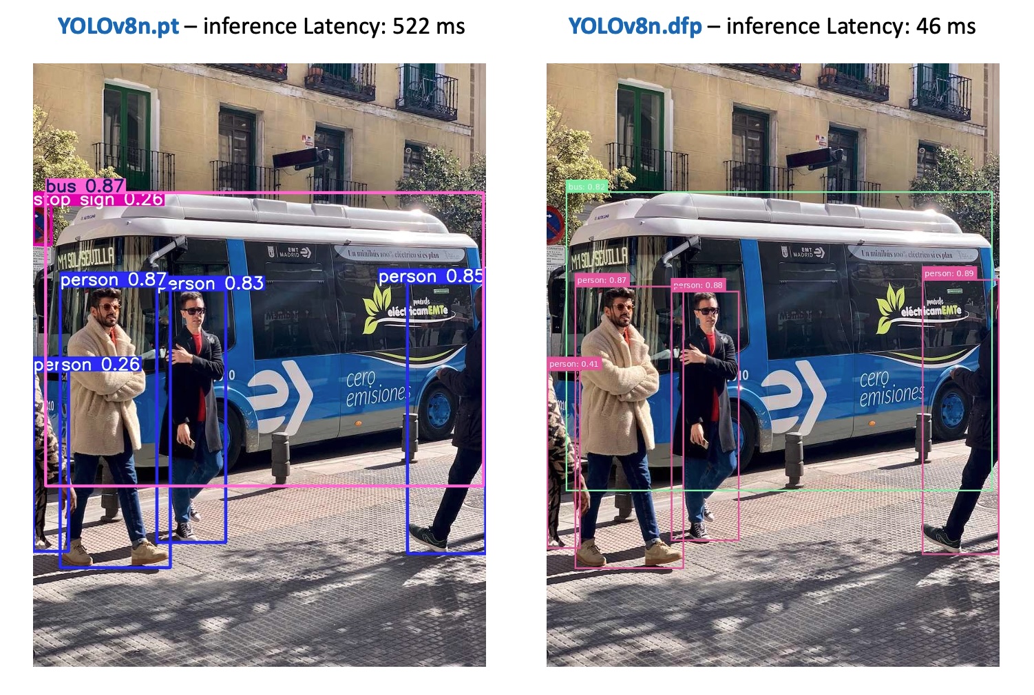
yolo predict model='yolov8n' source='https://ultralytics.com/images/bus.jpg'

The model and the image bus.jpg will be download and tested with the YOLOV8n:

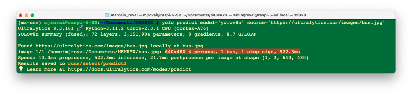
4 persons, 1 bus, and one stop signal were detected in 522 ms.

Under ./runs/detect, the output processed image can be analysed:

Model Export and Compilation

Step 1: Export YOLOv8 to ONNX

YOLOv8 must be converted to ONNX format before compilation for the MX3:

from ultralytics import YOLO

#### Load pretrained YOLOv8n model
model = YOLO('yolov8n.pt')

#### Export to ONNX format
model.export(format='onnx', simplify=True)

This creates yolov8n.onnx with the complete model graph.

We can also use CLI for the conversion:

yolo export model=yolov8n.pt format=onnx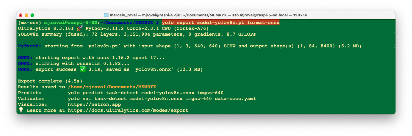

Step 2: Compile for MX3

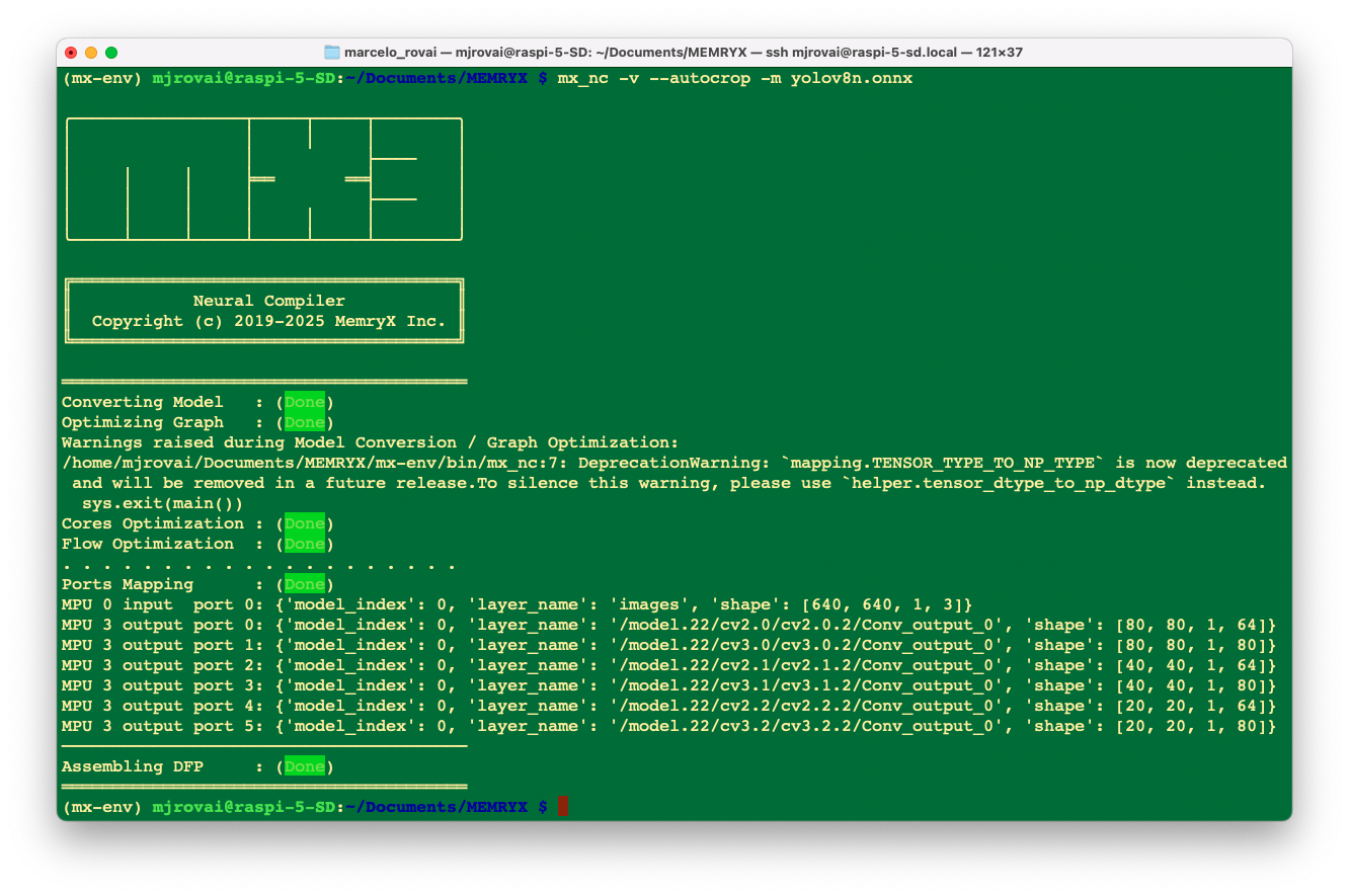
We can use the MemryX Neural Compiler to generate the DFP file:

mx_nc -v --autocrop -m yolov8n.onnx

Key flags:

-v: Verbose output for debugging
-m: Input model path
--autocrop: Automatically split model for optimal MX3 execution

Output files:

yolov8n.dfp - Accelerator executable (runs on MX3 chips)
yolov8n_post.onnx - Post-processing model (runs on CPU)

Why Two Files?

The MX3 compiler splits the model:

Feature extraction (yolov8n.dfp): Neural network backbone on MX3 hardware
Detection head (yolov8n_post.onnx): Bounding box decoding on CPU

This hybrid approach optimizes performance by running computationally intensive operations on the accelerator while keeping final post-processing flexible.

Now, let’s check the model with a benchmark

mx_bench -d yolov8n.dfp -f 1000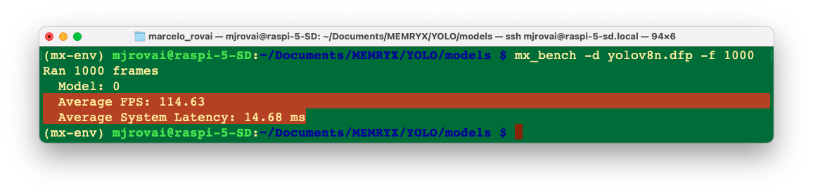

Understanding YOLOv8 Output Format

YOLOv8 Output Structure

The post-processing model outputs predictions in shape (1, 84, 8400):

Dimension 0 (1): Batch size
Dimension 1 (84):
- First 4 values: Bounding box [x_center, y_center, width, height]
- Next 80 values: Class probabilities (COCO dataset)
Dimension 2 (8400): Anchor points across three detection scales:
- 80×80 = 6400 points (small objects)
- 40×40 = 1600 points (medium objects)
- 20×20 = 400 points (large objects)

Decoding Process

Transpose: Convert from (1, 84, 8400) → (8400, 84)
Extract: Separate boxes and class scores
Filter: Keep predictions above confidence threshold
Convert coordinates: Transform from xywh to xyxy
NMS: Remove overlapping detections
Scale: Map to original image coordinates

Complete Inference Pipeline

We should now create a script to run an object detector (YOLOv8 with a pre/post-processing pipeline), print each detection (label, confidence, bounding box), and save a copy of the image with the boxes drawn.

Configuration section

At the top of __main__ we define the configuration values:

DFP_PATH = "./models/yolov8n.dfp"
POST_MODEL_PATH = "./models/yolov8n_post.onnx"
IMAGE_PATH = "./images/bus.jpg"
CONF_THRESHOLD = 0.25

DFP_PATH: path to the compiled model used for inference.
POST_MODEL_PATH: path to a post-processing model or graph, usually converting raw outputs into boxes, scores, and class IDs.
IMAGE_PATH: image file we want to run detection on.
CONF_THRESHOLD: minimum confidence score; detections below this are filtered out.

Running detection

detections, annotated_image, inference_time = detect_objects(
    DFP_PATH,
    POST_MODEL_PATH,
    IMAGE_PATH,
    CONF_THRESHOLD
)

Here we call a helper function detect_objects that encapsulates the heavy lifting:

Loads the model(s).
Loads and preprocesses the image.
Runs inference.
Applies post-processing (NMS, thresholding, etc.).
Returns:
- detections: list/array where each element is [x1, y1, x2, y2, conf, class_id].
- annotated_image: a PIL image with bounding boxes and labels drawn.
- inference_time: time spent doing the detection (in milliseconds).

Printing results

print(f"\n{'='*60}")
print("Detection Results:")
print(f"{'='*60}")
for i, det in enumerate(detections):
    x1, y1, x2, y2, conf, class_id = det
    print(f"  {i+1}. {COCO_CLASSES[int(class_id)]}: {conf:.3f}")
    print(f"      Box: [{int(x1)}, {int(y1)}, {int(x2)}, {int(y2)}]")

The loop goes over each detection, unpacks the bounding box coordinates, confidence, and class ID.
COCO_CLASSES[int(class_id)] converts the numeric class index into a human-readable label (e.g., “person”, “bus”).
Coordinates are cast to int for cleaner printing.

Saving the annotated image

if len(detections) > 0:
    output_path = IMAGE_PATH.rsplit('.', 1)[0] + '_detected.jpg'
    annotated_image.save(output_path)
    print(f"\nSaved: {output_path}")

Only saves an output file if at least one object was detected.
The output filename is built by taking the original name and appending _detected before the extension (e.g., bus_detected.jpg).
annotated_image.save(...) writes the image with drawn boxes and labels to disk.

Final summary output

print(f"\n{'='*60}")
print(f"Total: {len(detections)} objects")
print(f"Time: {inference_time:.2f} ms")
print(f"{'='*60}")

Prints how many objects were found in total.
Prints the inference time, which is useful to talk about performance (e.g., model size vs. speed, hardware differences).

Run the script yolov8_m3_detect.py

python yolov8_m3_detect.py

As a result, we can see that the models found 4 persons and 1 bus, missing only the stop signal. Regarding latency, the MX3 runs inference about 11 times faster than a CPU-only system.

Basically, the same accuracy result that we got on the YOLO chapter running yolov11

Going deeper in the functions

1. Image preprocessing (`preprocess_image`)

original image → resized → padded → tensor

Load and normalize:
- Open the image with PIL, convert to RGB, and get its original size.
- Compute a scale ratio so the image fits into 640×640 without distortion (preserving aspect ratio).
Letterboxing:
- Resize the image to (new_w, new_h) = (int(w * ratio), int(h * ratio)).
- Paste it onto a 640×640 canvas filled with color (114, 114, 114) (same as Ultralytics).
- Compute the padding offsets (pad_w, pad_h) so we can undo this later.
Tensor conversion:
- Convert to numpy, normalize to [0,1], permute from HWC to CHW, and add a batch dimension to get shape [1, 3, 640, 640], which matches YOLOv8’s expected input.[1][2]

2. Decoding YOLOv8 output (`decode_predictions`)

How to turn raw model numbers into human-readable detections.

The raw output format:

For COCO YOLOv8n ONNX, the detection head outputs a tensor of shape (1, 84, 8400).
84 = 4 (bbox) + 80 (class scores). Each of the 8400 positions corresponds to one candidate box.

Function Walkthrough:

Transpose:
- From (1, 84, 8400) to (8400, 84) so each row is: [x_center, y_center, width, height, class_0_score, ..., class_79_score].
Best class per box:
- Take max_scores = np.max(class_scores, axis=1) and class_ids = np.argmax(class_scores, axis=1) to select the most likely class and its score for each of the 8400 candidates.
Confidence filtering:
- Drop boxes whose max class score is below conf_threshold.
Coordinate conversion:
- Convert from YOLO’s center-format (x, y, w, h) to corner-format (x1, y1, x2, y2) to make drawing and IoU calculation simpler.
NMS:
- Call apply_nms to remove overlapping boxes and keep only the best ones.

3. IoU and NMS (`compute_iou_batch` and `apply_nms`)

IoU:

IoU (Intersection over Union) measures overlap between two boxes:
\[\text{IoU} = \frac{\text{area of intersection}}{\text{area of union}}\]
compute_iou_batch does this between one box and many boxes at once using vectorized Numpy operations.

NMS:

apply_nms:
- Sort boxes by score descending.
- Repeatedly pick the highest-score box, compute its IoU with the remaining boxes, and discard those whose IoU is above iou_threshold.
The result is a list of indices for boxes that don’t overlap too much and represent unique objects.

4. Mapping back to the original image (`scale_boxes_to_original`)

Everything after the model must undo what preprocessing did.

During preprocessing we:
- Rescaled the image by ratio.
- Padded by (pad_w, pad_h).
The model’s boxes live in that padded, resized 640×640 space.
scale_boxes_to_original:
- Subtracts the padding.
- Divides by ratio to go back to the original resolution.
- Clips coordinates so they stay inside the original image bounds.

5. Drawing results (`draw_detections`)

model output → decoded boxes → drawn on the original image

Make a copy of the original image and get an ImageDraw context.
For each detection:
- Choose a color deterministically using np.random.seed(class_id) so the same class always has the same color.
- Draw the rectangle [x1, y1, x2, y2].
- Build a label string "class_name: confidence", measure text size using textbbox, draw a filled rectangle for the label background, and render the text.

6. The Memryx pipeline (`detect_objects` and `AsyncAccl` usage)

How to integrate Memryx’s async accelerator into a typical vision pipeline

Preprocess once: call preprocess_image to get the model-ready tensor and the info needed for rescaling.
Create the accelerator:
- accl = AsyncAccl(dfp_path) loads the compiled Memryx DFP model.
- accl.set_postprocessing_model(post_model_path, model_idx=0) attaches the ONNX post-processing graph.
Streaming-style design:
- frame_queue is a queue of inputs; you put your tensor in it.
- generate_frame is a generator feeding frames into the accelerator.
- process_output is a callback that collects outputs into results.
- The code wires them with connect_input and connect_output, then waits for completion with accl.wait().
Post-processing:
- Grab the first output, call decode_predictions, rescale boxes, and draw.

Making Inferences

Let’s change the script to easily handle different images and confidence threshold (yolov8_m3_detect_v2.py). We should replace the hardcoded IMAGE_PATH with a command-line argument:

import argparse

if __name__ == "__main__":
    parser = argparse.ArgumentParser()
    parser.add_argument(
        "-i", "--image",
        type=str,
        required=True,
        help="Path to input image"
    )
    parser.add_argument(
        "-c", "--conf",
        type=float,
        default=0.25,
        help="Confidence threshold"
    )
    args = parser.parse_args()

    # Configuration
    DFP_PATH = "./models/yolov8n.dfp"
    POST_MODEL_PATH = "./models/yolov8n_post.onnx"
    IMAGE_PATH = args.image
    CONF_THRESHOLD = args.conf

    # Run detection
    detections, annotated_image, inference_time = detect_objects(
        DFP_PATH,
        POST_MODEL_PATH,
        IMAGE_PATH,
        CONF_THRESHOLD
    )

    # Print results
    print(f"\n{'='*60}")
    print("Detection Results:")
    print(f"{'='*60}")
    for i, det in enumerate(detections):
        x1, y1, x2, y2, conf, class_id = det
        print(f"  {i+1}. {COCO_CLASSES[int(class_id)]}: {conf:.3f}")
        print(f"      Box: [{int(x1)}, {int(y1)}, {int(x2)}, {int(y2)}]")

    # Save annotated image
    if len(detections) > 0:
        output_path = IMAGE_PATH.rsplit('.', 1)[0] + '_detected.jpg'
        annotated_image.save(output_path)
        print(f"\nSaved: {output_path}")

    print(f"\n{'='*60}")
    print(f"Total: {len(detections)} objects")
    print(f"Time: {inference_time:.2f} ms")
    print(f"{'='*60}")

We can run it as:

python yolov8_mx3_detect_v2.py --image ./images/home-office.jpg -c 0.2

Here are some results with other images:

Inference with a custom model

As we saw in the YOLO chapter, we are assuming we are in an industrial facility that must sort and count wheels and special boxes.

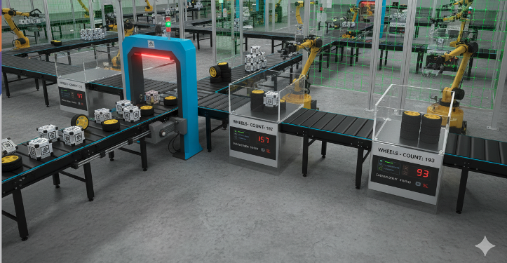
Each image can have three classes:

Background (no objects)
Box
Wheel

We have captured a raw dataset using the Raspberry Pi Camera and labeled it with the ROBOFLOW. The Yolo model was trained on a Google Colab using Ultralytics.

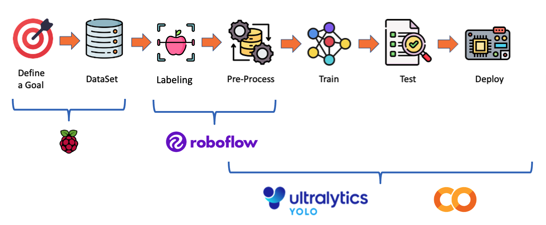
After training, we download the trained model from /runs/detect/train/weights/best.pt to our computer, renaming it to box_wheel_320_yolo.pt.

Using the FileZilla FTP, transfer a few images from the test dataset to .\images:

Let’s return to the ./MEMRYX/YOLO folder and using the Python Interpreter, to quickly do some inferences:

python

We will import the YOLO library and define the model to use:

>>> from ultralytics import YOLO
>>> model = YOLO('./models/box_wheel_320_yolo.pt')

Now, let’s define an image and call the inference (we will save the image result this time to external verification):

>>> img = './images/box_3_wheel_4.jpg'
>>> result = model.predict(img, save=True, imgsz=320, conf=0.5, iou=0.3)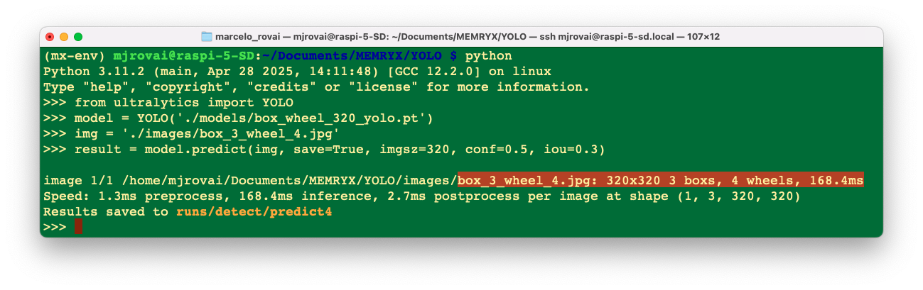

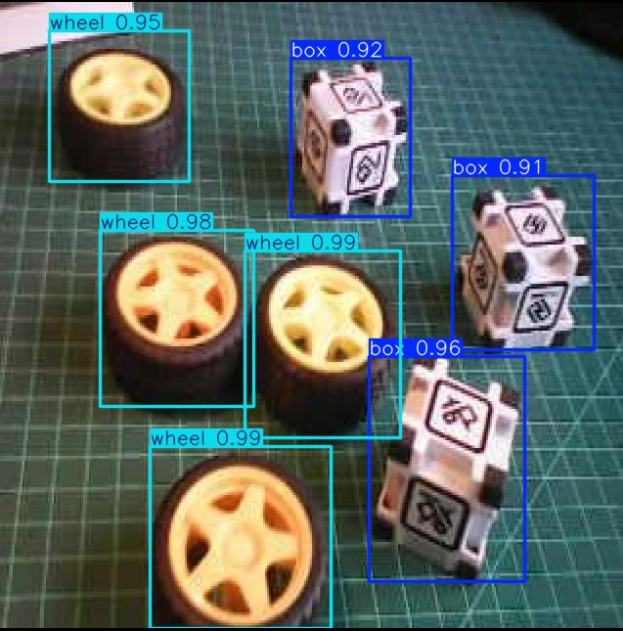
We can see that the model is working and that the latency was 168 ms.

Let’s now export the model first to ONNX and after to FFPls

, to run it in the MX3 device:

cd ./models
yolo export model=box_wheel_320_yolo.pt format=onnx
mx_nc -v --autocrop -m box_wheel_320_yolo.onnx
cd ..

In the models folder, we will have box_wheel_320_yolo.dfp and box_wheel_320_yolo_post.onnx

Let’s adapt the previous script to be more generic in terms of models (box_wheel_mx3_detect_v2.py):

Naturally we should enter with the new models ’names and instead of COCO_LABELS, the script was changed to:
# dataset class names 
CLASSES = [
    'Box', 'Wheel'
]
Thant’s all!

Run it with:

python box_wheel_mx3_detect_v2.py --image ./images/box_3_wheel_4.jpg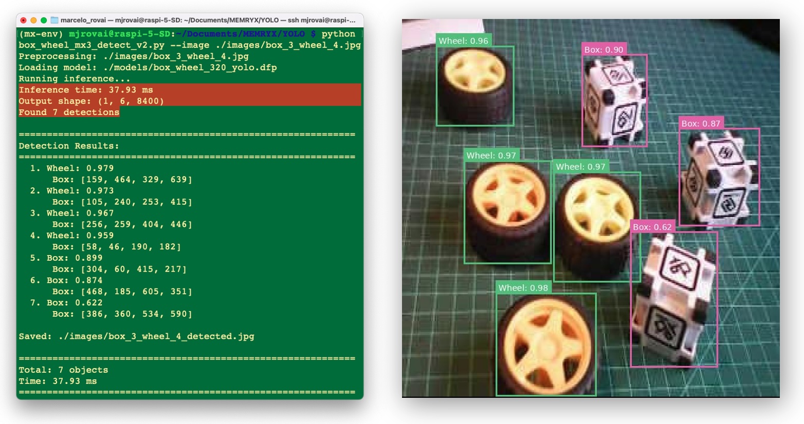

The Result was great! And the latency (~38 ms) was 4 times lower than with the CPU-only approach (even smaller than the model exported to NCNN, runing 100% at CPU - 80 ms).

Adjusting Confidence Threshold

Lower confidence for more detections (may include false positives):

python box_wheel_mx3_detect_v2.py --image ./images/box_3_wheel_4.jpg -c 0.15

We should experiment with the right confidence threshold.

Advanced Topics

Batch Processing (Optimization)

For multiple images, reuse the accelerator instance:

accl = AsyncAccl(dfp_path)
accl.set_postprocessing_model(post_model_path)

for image_path in image_list:
    detections = detect_single_image(accl, image_path)

Thermal Management

Always monitor temperature during operation:

watch -n 1 cat /sys/memx0/temperature

Confidence Threshold Tuning

0.15-0.20: Maximum recall (catch everything)
0.25-0.40: Balanced (default)
0.45-0.50: High precision (only confident detections)

Model Selection

yolov8n: Fastest, 3.2M parameters
yolov8s: Balanced, 11.2M parameters
yolov8m: Accurate, 25.9M parameters

Exploring MemryX eXamples

MemryX eXamples is a collection of end-to-end AI applications and tasks powered by MemryX hardware and software solutions. These examples provide practical, hands-on use cases to help leverage MemryX technology.

Clone the MemryX eXamples Repository

Clone this repository plus any linked submodules:

git clone --recursive https://github.com/memryx/memryx_examples.git
cd memryx_examples

After cloning the repository, you’ll find several subdirectories with different categories of applications:

image_inference - Single image classification and detection
video_inference - Real-time video processing
multistream_video_inference - Multi-camera scenarios
audio_inference - Audio processing and speech recognition
open_vocabulary - Open-set classification tasks
accuracy_calculation - Model accuracy verification
multi_dfp_application - Running multiple models
optimized_multistream_apps - Production-ready multi-stream examples
fun_projects - Creative applications and demos

These examples demonstrate best practices for:

Preprocessing pipelines
Multi-threaded inference
Output visualization
Performance optimization
Multi-model orchestration

Exploring these examples is an excellent way to learn production-ready patterns for deploying MemryX applications.

Troubleshooting Common Issues

Device Not Detected

Symptom: ls /dev/memx* returns “No such file or directory”

Solutions:

Verify physical connection: Reseat the M.2 module in its slot
Check PCIe settings:

sudo raspi-config
# Navigate to: Advanced Options → PCIe Speed → Enable PCIe Gen 3
sudo reboot

Verify in kernel logs:

dmesg | grep -i memryx
lspci | grep -i memryx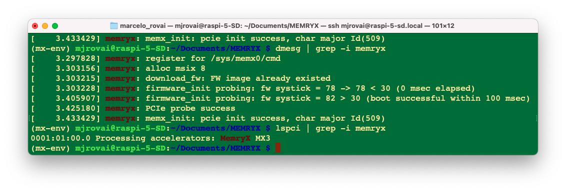

Ensure sufficient power: Use the official Raspberry Pi 27W power supplyCheck HAT installation: Ensure the M.2 HAT is properly seated.
Lower Frequency: Try running sudo mx_set_powermode with a lower frequency, such as 200 or 300 MHz. Then restart mxa-manager for good measure with sudo service mxa-manager restart

sudo mx_set_powermode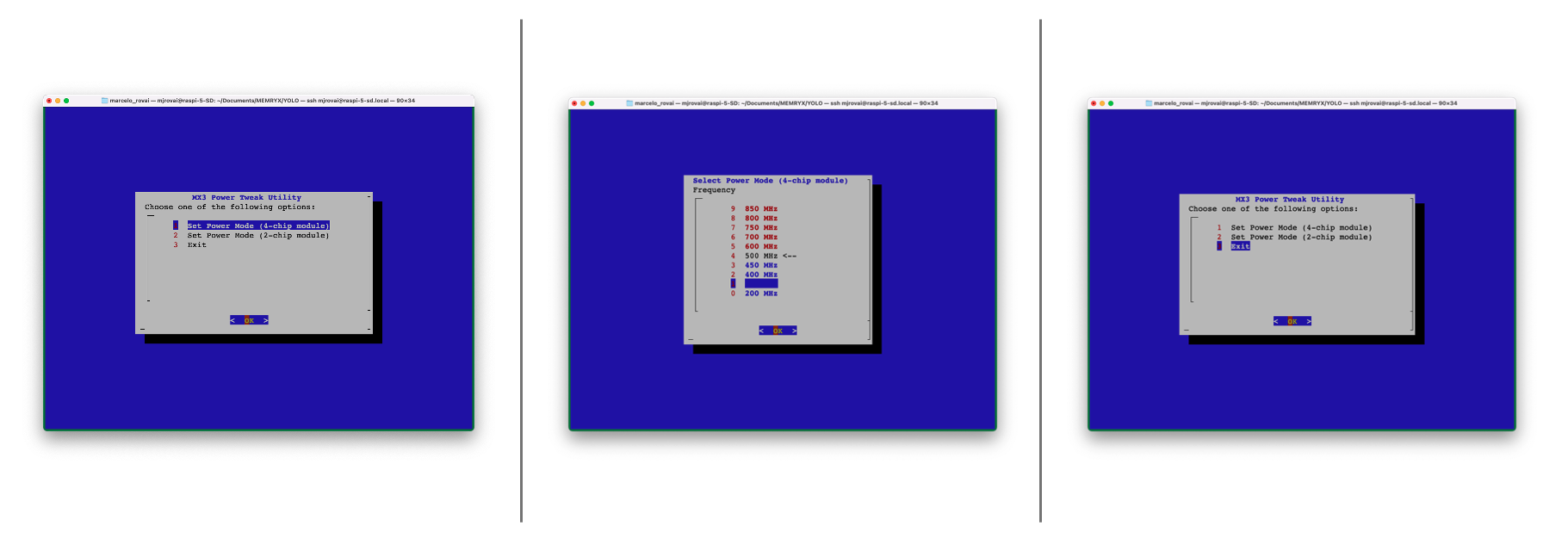

sudo service mxa-manager restart

Check the frequency with the following command:

cat /etc/memryx/power.conf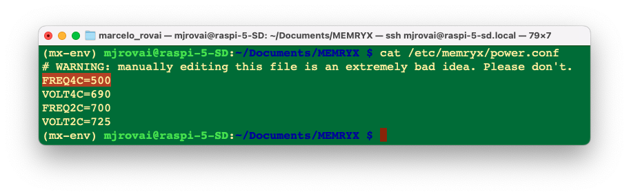

We can check it by the first field of the file, FREQ4. If the Raspberry Pi is set to the module’s default operating frequency (500 MHz), we should see FREQ4C=500, indicating that the module is set to a 500 MHz clock speed for 4-chip DFPs.

If decreasing the frequency solves the issue, then you can either keep the default frequency for all DFPs at 300 MHz (or 400, 450, etc.), or you can raise it back to 500 MHz and use the C++ API’s set_operating_frequency function to change the clock speed on a per-DFP basis.

Compilation Errors

Symptom: mx_nc fails with “Unsupported operator” error

Solutions: - Check the supported operators

Some custom layers may need reformulation
Try exporting to ONNX first for better compatibility:

import tensorflow as tf
import tf2onnx

model = tf.keras.models.load_model('model.h5')
onnx_model, _ = tf2onnx.convert.from_keras(model)
with open("model.onnx", "wb") as f:
    f.write(onnx_model.SerializeToString())

Check the compilation log (-v flag) to identify which specific layer is causing issues

Thermal Throttling

Symptom: Performance degrades over time, temperature > 90°C

Solutions:

Verify heatsink installation: Ensure thermal paste is properly applied and heatsink is firmly attached
Improve airflow: Position the Raspberry Pi for better air circulation
Check ambient temperature: Ensure the room temperature is reasonable (<30°C)
Monitor continuously:

watch -n 1 cat /sys/memx0/temperature

= Consider additional cooling: Add a small fan directed at the heatsink

Python Version Conflicts

Symptom: pip install memryx fails with compatibility errors

Solutions:

Verify Python version:

python --version  # Must show 3.11.x or 3.12.x
pip --version     # Should match the Python version

Ensure you’re in the virtual environment:

which python  # Should point to mx-env/bin/python

Try reinstalling in a fresh virtual environment:

deactivate
rm -rf mx-env
python -m venv mx-env
source mx-env/bin/activate
pip install --upgrade pip wheel
pip install --extra-index-url https://developer.memryx.com/pip memryx

Low FPS / Poor Performance

Symptom: Benchmark shows much lower FPS than expected

Solutions:

Check for thermal throttling:

cat /sys/memx0/temperature  # Should be <80°C

Verify PCIe Gen 3 is enabled (not Gen 2):

sudo raspi-config
# Advanced Options → PCIe Speed

Close other PCIe-intensive applications: Ensure no other devices are saturating the PCIe bus
Check for background CPU load:

htop

Verify driver version: Ensure you have the latest drivers

apt policy memx-drivers

Verify Frequency

By default, the frequency should be at 500 MHz. Smaller frequencies will reduce the FPS (increase the latency)

cat /etc/memryx/power.conf

Import Errors

Symptom: ImportError: cannot import name 'SyncAccl' from 'memryx'

Solutions:

Ensure memryx is installed in the current environment:

pip list | grep memryx

Reinstall if necessary:

pip install --force-reinstall --extra-index-url \
https://developer.memryx.com/pip memryx

Check Python path conflicts:

import sys
print(sys.path)

Model Accuracy Issues

Symptom: Inference results are incorrect or significantly different from CPU

Solutions: - Verify preprocessing: Ensure the same preprocessing is applied as during training

Check input normalization: Confirm the value range matches training (e.g., [0, 1] vs [-1, 1])
Test with known inputs: Use the validation dataset to verify accuracy
Compare outputs numerically: Print raw logits/probabilities to identify differences
Check for quantization effects: If using -q flag, try without quantization first

Next Steps and Extensions

Project Ideas

Real-time Object Detection with Camera
- Integrate picamera2 with YOLO
- Display bounding boxes in real-time
- Measure end-to-end latency (capture → inference → display)
Multi-Model Pipeline
- Use detection + classification cascade
- Leverage multiple MX3 chips for parallel inference
- Build a smart surveillance system
Custom Model Deployment
- Train your own model for a specific task
- Optimize and compile for MX3
- Compare against the models from previous labs
Power Efficiency Study
- Measure power consumption with a USB meter
- Compare CPU vs. MX3 energy per inference
- Calculate battery life for mobile applications
Multi-Stream Processing
- Process multiple camera streams simultaneously
- Demonstrate chip utilization across streams
- Build a multi-camera monitoring system

Advanced Topics to Explore

Quantization: Experiment with 8-bit and 4-bit quantization for even better performance
Model Zoo: Explore pre-optimized models in the MemryX Model Explorer
Async API: Use AsyncAccl for non-blocking, concurrent processing
Custom Operators: Learn to handle models with custom layers
Multi-chip Scaling: Understand how workload distributes across the four accelerators

Conclusion

In this lab, we’ve explored hardware acceleration for edge AI using the MemryX MX3 accelerator. We’ve learned:

✅ How to install and configure the MX3 hardware
✅ The MX3 compilation and deployment workflow
✅ How to benchmark and measure performance
✅ Building complete inference applications
✅ Comparing CPU vs. dedicated accelerator performance

The MX3 demonstrates that dedicated AI accelerators can deliver significant performance improvements for edge applications, achieving FPS several times higher (up to 25x for ResNet-50) than CPU inference while maintaining accuracy and providing deterministic latency.

As edge AI continues to evolve, hardware acceleration will become increasingly important for real-time, power-efficient deployments. The skills we’ve developed in this lab—understanding the compilation workflow, benchmarking methodologies, and performance optimization—will transfer to other accelerator platforms as well.

Introduction

Why Hardware Acceleration?

Our goal

Hardware Installation and Verification

Prerequisites

Installation and Cooling Considerations

Verification

Software Installation

Create Project Directory

Python Version Management with Pyenv

Installing Pyenv on Debian Trixie

Set Python Version for Project

MemryX Drivers and SDK Installation

Prepare the System

Add MemryX Repository and Key

Update and Install Drivers and SDK

Configure Platform Settings

Verify Driver Installation

Install Utilities

Prepare System Dependencies

Install Tools (Inside Virtual Environment)

Verification

Our First Accelerated Model

Understanding the MX3 Workflow

Step 1: Select or Train a Model

Step 2: Compile with Neural Compiler

Step 3: Deploy and Benchmark

Step 4: Integrate into the Application

Complete Workflow Example

Download and Compile MobileNetV2

What is a DFP file?

Benchmarking Performance

Building an Inference Application

Prepare Directory Structure

Download Test Image

Understanding Input Requirements

Getting the Labels

Image Preprocessing

Prepare Input Tensor

Run Inference on MemryX Accelerator (MXA)

Decode the MXA Results

Comparing CPU vs. MXA Performance

Measuring Latency

Testing with Larger Models

Clean Shutdown

Folders Structure

Performance Comparison Summary

Key Observations

When to Use the MX3?

YOLOv8 Object Detection with MX3 Hardware Acceleration

Model Export and Compilation

Step 1: Export YOLOv8 to ONNX

Step 2: Compile for MX3

Understanding YOLOv8 Output Format

YOLOv8 Output Structure

Decoding Process

Complete Inference Pipeline

Configuration section

Running detection

Printing results

Saving the annotated image

Final summary output

Going deeper in the functions

1. Image preprocessing (preprocess_image)

2. Decoding YOLOv8 output (decode_predictions)

3. IoU and NMS (compute_iou_batch and apply_nms)

4. Mapping back to the original image (scale_boxes_to_original)

5. Drawing results (draw_detections)

6. The Memryx pipeline (detect_objects and AsyncAccl usage)

Making Inferences

Inference with a custom model

Adjusting Confidence Threshold

Advanced Topics

Batch Processing (Optimization)

Thermal Management

Confidence Threshold Tuning

Model Selection

Exploring MemryX eXamples

Clone the MemryX eXamples Repository

Troubleshooting Common Issues

1. Image preprocessing (`preprocess_image`)

2. Decoding YOLOv8 output (`decode_predictions`)

3. IoU and NMS (`compute_iou_batch` and `apply_nms`)

4. Mapping back to the original image (`scale_boxes_to_original`)

5. Drawing results (`draw_detections`)

6. The Memryx pipeline (`detect_objects` and `AsyncAccl` usage)