Physical Computing with Raspberry Pi
From Sensors to Smart Analysis with Small Language Models

Introduction
Physical computing creates interactive systems that sense and respond to the analog world. While this field has traditionally focused on direct sensor readings and programmed responses, we’re entering an exciting new era where Large Language Models (LLMs) can add sophisticated decision-making and natural language interaction to physical computing projects.
In the Small Language Models (SLM) chapter, we learned how to run an LLM (or, more precisely, an SLM) on a Single Board Computer (SBC) such as the Raspberry Pi. In this chapter, we will go through the process of setting up a Raspberry Pi for physical computing, with an eye toward future AI integration. We’ll cover:
- Setting up the Raspberry Pi for physical computing
- Working with essential sensors and actuators
- Understanding GPIO (General Purpose Input/Output) programming
- Establishing a foundation for integrating LLMs with physical devices
- Creating interactive systems that can respond to both sensor data and natural language commands
We will also use a Jupyter notebook (programmed in Python) to interact with sensors and actuators—an important and necessary first step toward the goal of integrating the Raspi with an SLM.
The combination of Raspberry Pi’s versatility and the power of SLMs opens up exciting possibilities for creating more intelligent and responsive physical computing systems.
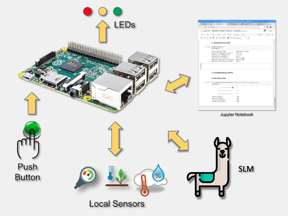
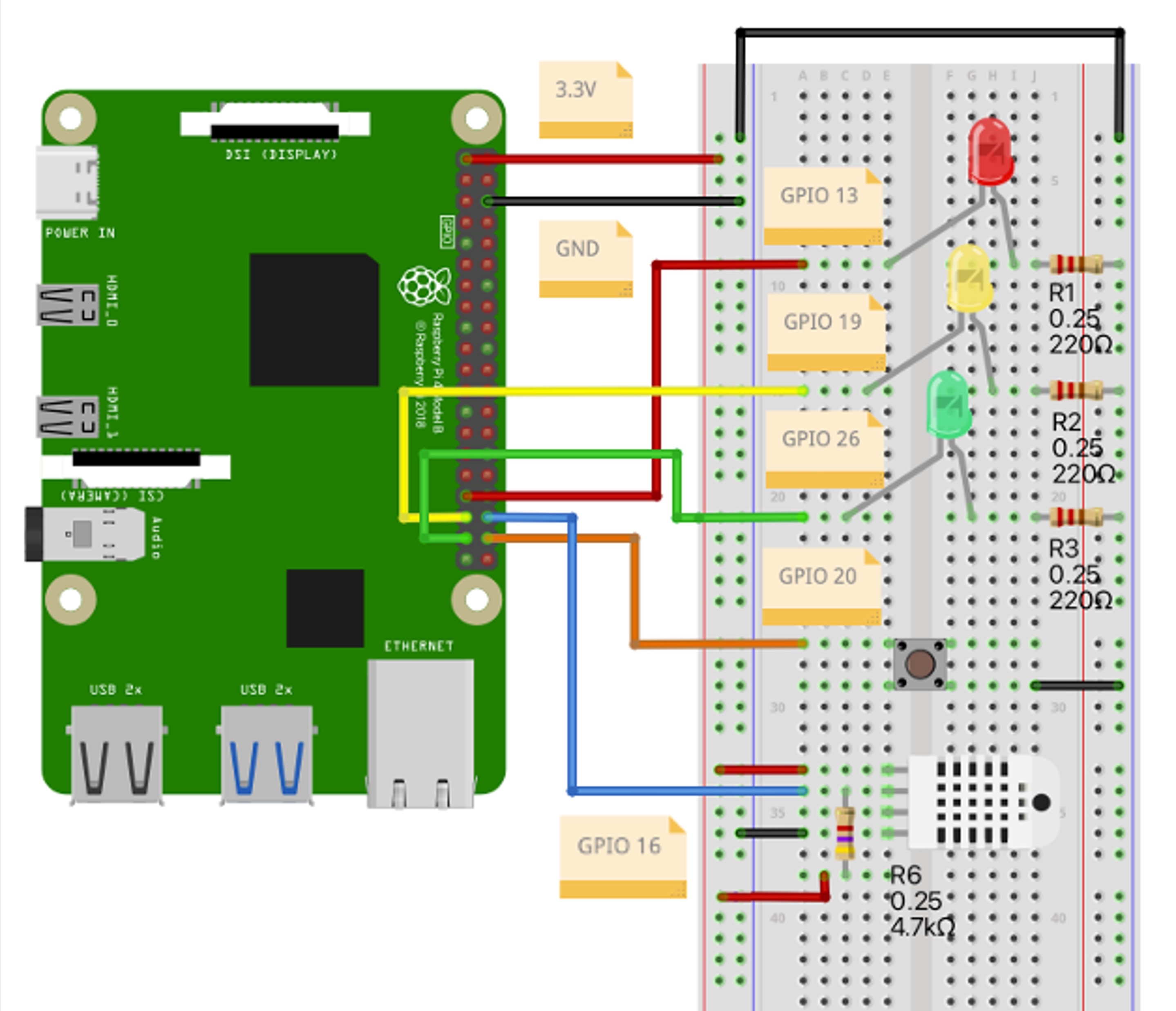
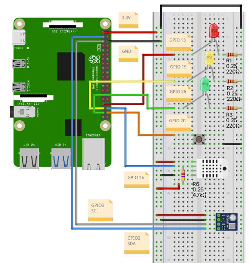
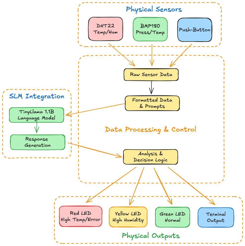
The diagram below gives us an overview of the project:
Prerequisites
- Raspberry Pi (model 4 or 5)
- DHT22 Temperature and Relative Humidity Sensor
- BMP280 Barometric Pressure, Temperature and Altitude Sensor
- Colored LEDs (3x)
- Push Button (1x)
- Resistor 4K7 ohm (2x)
- Resistor 220 or 330 ohm (3x)
Accessing the GPIOs
The Raspberry Pi’s GPIO (General Purpose Input/Output) pins allow us to connect electronic components and control them with Python code. This opens up endless possibilities for creating interactive projects, home automation systems, robotics, and more.
This chapter covers the modern GPIO Zero library for interactions with buttons and LEDs.
⚠️ IMPORTANT: RPi.GPIO does NOT support Raspberry Pi 5!
With the Raspberry Pi 5, we must use GPIO Zero or the newer lgpio library. RPi.GPIO only works on Pi models 1-4, the Pi Zero, Pi Zero 2, and the Pi Zero 2W.
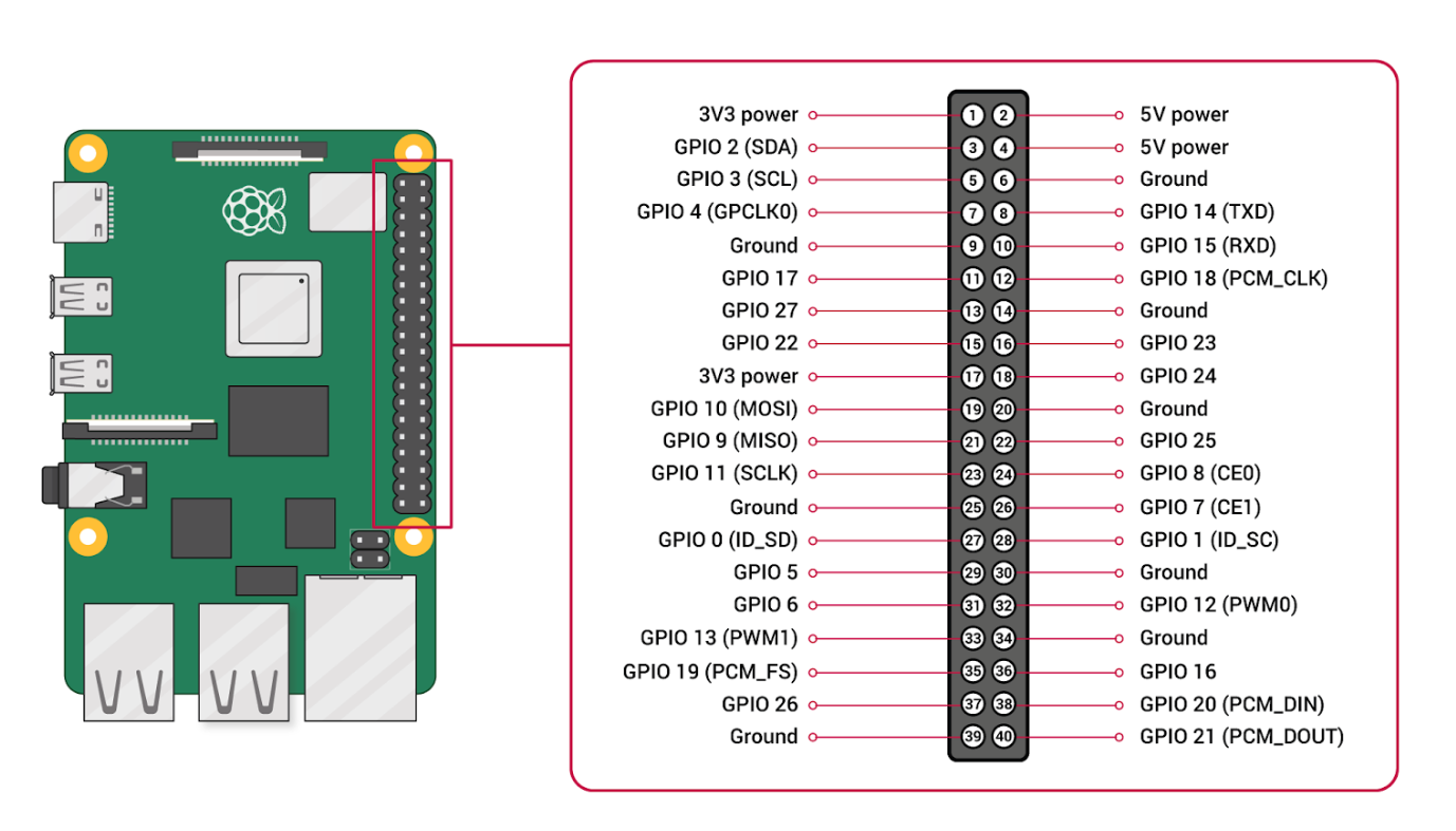
The Raspberry Pi has 40 pins on its header, but not all of them are GPIO pins. Some provide power (3.3V and 5V), others are ground pins, and the rest are programmable GPIO pins.
Pin Numbering Systems
There are two ways to reference GPIO pins:
BCM (Broadcom): Uses the GPIO number (e.g., GPIO17, GPIO27)
BOARD: Uses the physical pin number on the header (e.g., Pin 11, Pin 13)
In this chapter, we’ll use BCM numbering as it’s more commonly used in Python programming.
Safety First
Before connecting any components, please read these important safety guidelines:
Never connect 5V directly to GPIO pins - GPIO pins are 3.3V tolerant only
Always use current-limiting resistors with LEDs - Without them, you risk damaging the LED or GPIO pin
Double-check your connections before powering on
Disconnect power when making circuit changes
Respect polarity - LEDs for example, have positive (long leg) and negative (short leg) sides
GPIO Zero Library
A modern, high-level library that makes GPIO programming much simpler and more intuitive. It uses object-oriented programming and includes built-in features like automatic pin cleanup, device abstraction, and event detection.
It is essential to note that the GPIO Zero Library uses Broadcom (BCM) pin numbering for GPIO pins, rather than physical (board) numbering. Any pin marked “GPIO ” in the previous diagram can be used as a PIN. For example, if an LED were attached to
GPIO13, we would specify the PIN as13rather than 33 (the physical one).
It was created by Ben Nuttall of the Raspberry Pi Foundation, Dave Jones, and other contributors (GitHub).
Advantages of GPIO Zero:
Simpler, more readable code
Object-oriented approach (LED, Button, etc.)
Built-in device patterns and behaviors
Automatic cleanup on program exit
Better for beginners and rapid prototyping
Includes composite devices (robots, traffic lights, etc.)
Installation:
- GPIO Zero comes pre-installed on Raspberry Pi OS!
“Hello World”: Blinking an LED
Let’s start with the classic ‘Hello World’ of physical computing - making an LED blink!
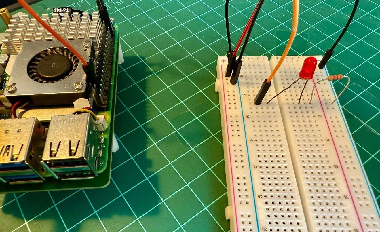
To connect our RPi to the world, let’s first connect:
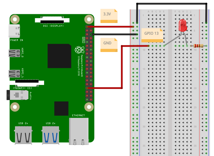
- Physical Pin 6 (GND) to GND Breadboard Power Grid (Blue -), using a black jumper
- Physical Pin 1 (3.3V) to +VCC Breadboard Power Grid (Red +), using a red jumper
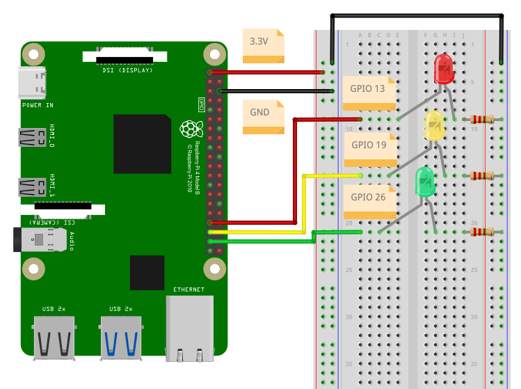
Now, let’s connect an LED (red) using the physical pin 33 (GPIO13) connected to the LED cathode (longer LED leg). Connect the LED anode to the breadboard GND using a 220 ohms resistor to reduce the current drawn from the Raspberry Pi, as shown below:
Understanding the LED Circuit
An LED (Light-Emitting Diode) requires current to flow through it to produce light. However, without a resistor, too much current can flow, damaging the LED or your Raspberry Pi. We use a resistor to limit the current to a safe level.
Why 220Ω or 330Ω Resistors?
These values limit the current to approximately 10-15mA, which is safe for most standard LEDs and GPIO pins. The exact value isn’t critical—anything from 220 Ω to 1 kΩ will work fine.
Testing with GPIO Zero
We can use the built-in Python interpreter to test the LED. In the terminal, enter python, and once in the interpreter, enter with the commands below:
python
>>> from gpiozero import LED
>>> led = LED(13)
>>> led.on()
>>> led.off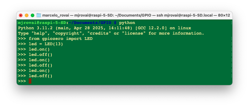
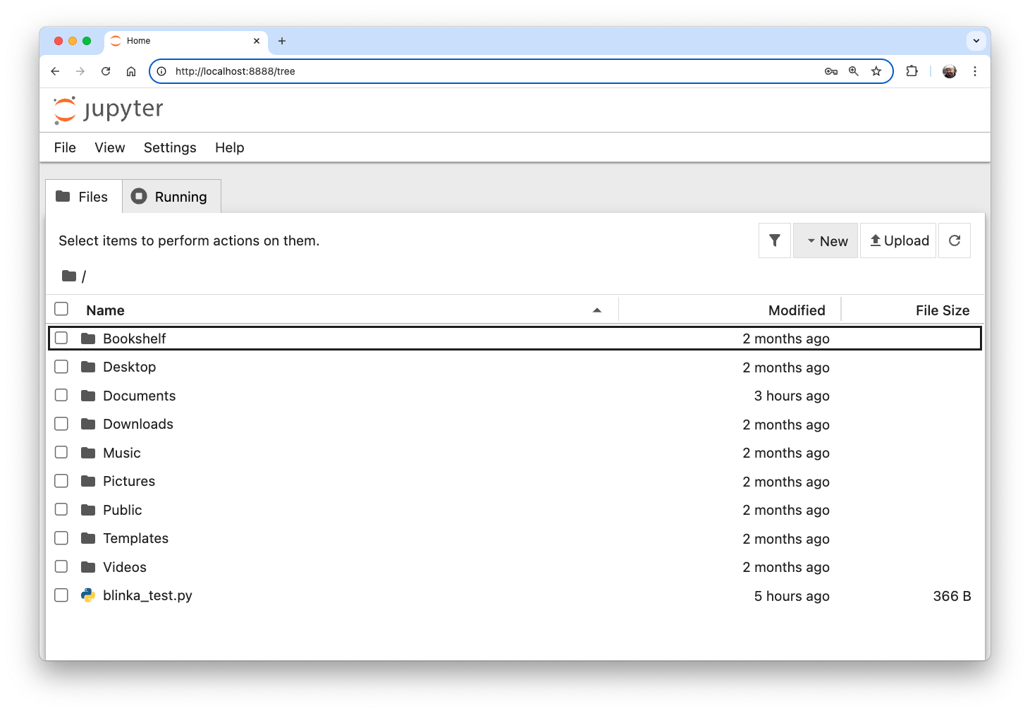
On the Raspberry, start at home and go to Documents.
cd DocumentsCreate a directory to save the scripts and install the libraries. Move to there:
mkdir GPIO
cd GPIO
We can use any text editor (such as Nano) to create and run the script. Save the file, for example, as led_test.py, and then execute it using the terminal:
python led_test.pyNow, let’s blink the LED (the actual “Hello world”) when talking about physical computing. To do that, we must also import another library: time. We need it to define how long the LED will be ON and OFF. In the case below, the LED will blink every 1 second.
from gpiozero import LED
from time import sleep
led = LED(13)
while True:
    led.on()
    sleep(1)
    led.off()
    sleep(1)
We can use any text editor (such as Nano) to create and run the script. Save the file, for example, as blink.py, and then execute it using the terminal:
python blink.pyAlternatively, we can reduce the blink code as below:
from gpiozero import LED
from signal import pause
led = LED(13)
led.blink() # 1 second by default
# led.blink(on_time=0.5, off_time=0.5) # Fast blink
pause()
Installing all LEDs (the “actuators”)
The LEDs can be used as “actuators”; depending on the condition of a code running on our Pi, we can command one of the LEDs to fire! We will install two more LEDs, in addition to the red one already installed. Follow the diagram and install the yellow (on GPIO 19 ) and the green (on GPIO 26).
For testing we can run a similar code as the used with the single red led, changing the pin accordantly, for example.
from gpiozero import LED
from time import sleep

ledRed = LED(13)
ledYlw = LED(19)
ledGrn = LED(26)

ledRed.off()
ledYlw.off()
ledGrn.off()

ledRed.on()
ledYlw.on()
ledGrn.on()

sleep(5)

ledRed.off()
ledYlw.off()
ledGrn.off()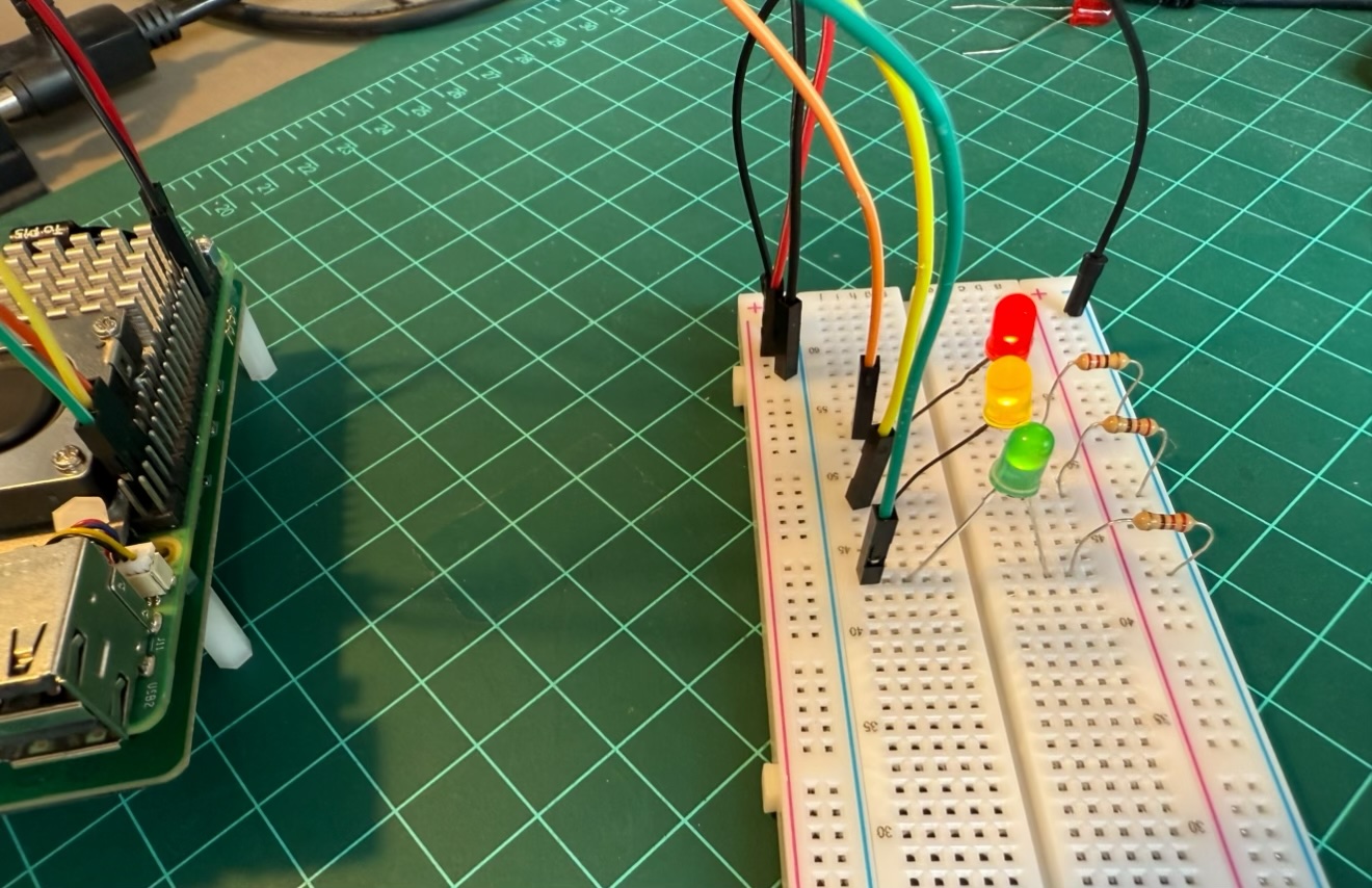
Remember that instead of LEDs, we could have relays, motors, etc.
Sensors Installation and setup
In this section, we will setup the Raspberry Pi to capture data from several different sensors:
Sensors and Communication type:
- Button (Command via a Push-Button) ==> Digital direct connection
- DHT22 (Temperature and Humidity) ==> Digital communication
- BMP280 (Temperature and Pressure) ==> I2C Protocol
Button
Now, let’s learn how to read input from a button. This allows your Raspberry Pi to respond to physical interactions!
Understanding Pull-Up and Pull-Down Resistors
When a button is not pressed, the GPIO pin is ‘floating’ - it’s not connected to anything and can read random values. We use pull-up or pull-down resistors to set the pin’s default state.
Pull-Down: Default state is LOW (0V), becomes HIGH when button pressed
Pull-Up: Default state is HIGH (3.3V), becomes LOW when button pressed
The Raspberry Pi has internal pull-up and pull-down resistors!
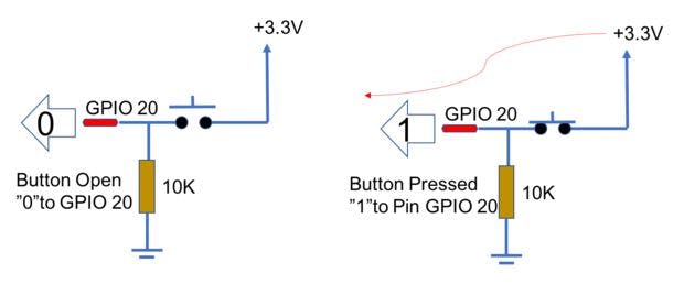
The simplest way to run an external command is with a push button, and the GPIO Zero Library makes it easy to include in the project. We do not need to think about Pull-up or Pull-down resistors, etc. In terms of HW, the only thing to do is to connect one leg of our push-button to any one of the Raspi GPIOs and the other one to GND, as shown in the diagram:
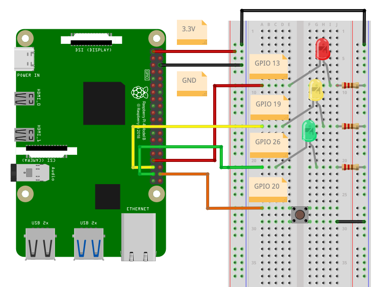
- Push-Button leg1 to GPIO 20
- Push-Button leg2 to GND
A simple code for reading the button can be:
from gpiozero import Button
button = Button(20)
while True:
    if button.is_pressed:
        print("Button is pressed")
    else:
        print("Button is not pressed")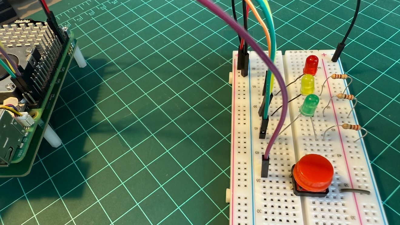
On a Raspberry Pi Zero 2W, for example, we could use the RPi.GPIO, whose code is:
import RPi.GPIO as GPIO
import time

GPIO.setmode(GPIO.BCM)
GPIO.setwarnings(False)

BUTTON_PIN = 20

# Set up with internal pull-up
GPIO.setup(BUTTON_PIN, GPIO.IN, pull_up_down=GPIO.PUD_UP)

try:
    while True:
        if GPIO.input(BUTTON_PIN) == GPIO.LOW:
            print('Button pressed!')
        else:
            print('Button not pressed')
        time.sleep(0.1)

except KeyboardInterrupt:
    GPIO.cleanup()
Installing Adafruit CircuitPython
The GPIO Zero library is an excellent hardware interfacing library for Raspberry Pi. It’s great for digital in/out, analog inputs, servos, basic sensors, etc. However, it doesn’t cover SPI/I2C sensors or drivers. By using CircuitPython via adafruit_blinka, we can take advantage of all of the drivers and example code developed by Adafruit!
Note that we will keep using GPIO Zero for pins, buttons, and LEDs.
Enable Interfaces
Run these commands to enable the various interfaces such as I2C and SPI:
sudo raspi-config nonint do_i2c 0
sudo raspi-config nonint do_spi 0
sudo raspi-config nonint do_serial_hw 0
sudo raspi-config nonint disable_raspi_config_at_boot 0
Install required dependencies
sudo apt-get install -y python3-libgpiod i2c-tools libgpiod-devInstall Blinka
Let’s enter the Ollama environment, alheady created to install Blinka:
source ~/ollama/bin/activateInstall the library
pip install adafruit-blinkaCheck I2C and SPI
The script will automatically enable I2C and SPI. You can run the following command to verify:
ls /dev/i2c* /dev/spi*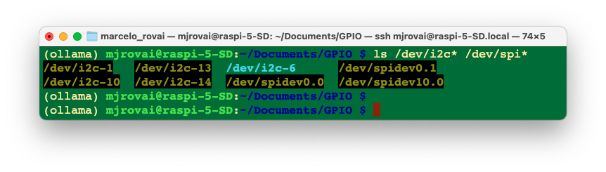
Verify Blinka Version
python3 -m pip show adafruit-blinka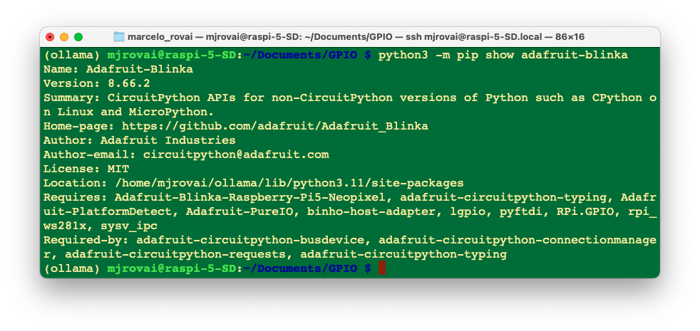
Blinka Installation Test
Create a new file called blinka_test.py with nano or your favorite text editor and put the following in:
import board
import digitalio
import busio

print("Hello, blinka!")

# Try to create a Digital input
pin = digitalio.DigitalInOut(board.D4)
print("Digital IO ok!")

# Try to create an I2C device
i2c = busio.I2C(board.SCL, board.SDA)
print("I2C ok!")

# Try to create an SPI device
spi = busio.SPI(board.SCLK, board.MOSI, board.MISO)
print("SPI ok!")

print("done!")
Save it and run it at the command line:
python blinka_test.py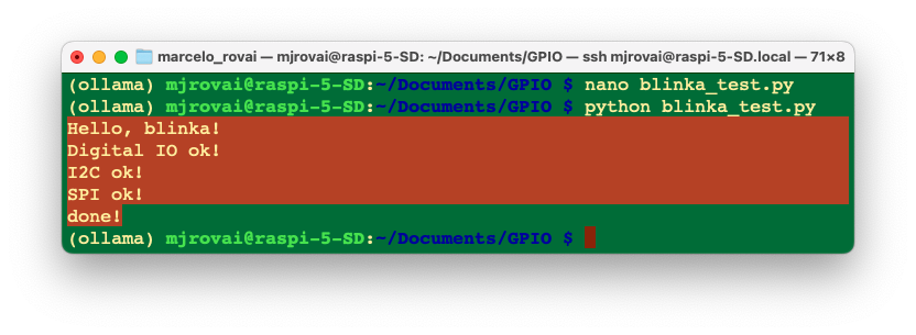
DHT22 - Temperature & Humidity Sensor
The first sensor to be installed will be the DHT22 for capturing air temperature and relative humidity data.
Overview
The low-cost DHT temperature and humidity sensors are elementary and slow, but great for logging basic data. They consist of a capacitive humidity sensor and a thermistor. A bare chip inside performs the analog-to-digital conversion and outputs a digital signal containing the temperature and humidity. The digital signal is relatively easy to read using any microcontroller.
DHT22 Main characteristics:
Suitable for 0-100% humidity readings with 2-5% accuracy
Suitable for -40 to 125°C temperature readings ±0.5°C accuracy
No more than 0.5 Hz sampling rate (once every 2 seconds)
Low cost
3 to 5V power and I/O
2.5mA max current use during conversion (while requesting data)
Body size 15.1mm x 25mm x 7.7mm
4 pins with 0.1” spacing
Once we use the sensor at distances less than 20m, a 4K7 ohm resistor should be connected between the Data and VCC pins. The DHT22 output data pin will be connected to Raspberry GPIO 16. Check the electrical diagram, connecting the sensor to RPi pins as below:
- Pin 1 - Vcc ==> 3.3V
- Pin 2 - Data ==> GPIO 16
- Pin 3 - Not Connect
- Pin 4 - Gnd ==> Gnd
Do not forget to Install the 4K7 ohm resistor between the VCC and Data pins.
Once the sensor is connected, we must install its library on our Raspberry Pi. First, we should install the Adafruit CircuitPython library, which we have already done, and the Adafruit_CircuitPython_DHT.
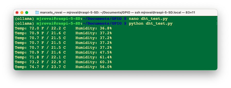
pip install adafruit-circuitpython-dhtCreate a new Python script as below and name it, for example, dht_test.py:
import time
import board
import adafruit_dht
dhtDevice = adafruit_dht.DHT22(board.D16)

while True:
    try:
        # Print the values to the serial port
        temperature_c = dhtDevice.temperature
        temperature_f = temperature_c * (9 / 5) + 32
        humidity = dhtDevice.humidity
        print(
            "Temp: {:.1f} F / {:.1f} C    Humidity: {}% ".format(
                temperature_f, temperature_c, humidity
            )
        )
        time.sleep(2.0)

    except RuntimeError as error:
        # Errors happen fairly often, DHT's are hard to read,
        # just keep going
        print(error.args[0])
        time.sleep(2.0)
        continue
    except Exception as error:
        dhtDevice.exit()
        raise error
Placing a finger on the sensor, we can see that both temperature and humidity begin to rise.
Addendum: DHT22 on Raspberry Pi 5 with Debian Trixie
adafruit_dht does not work
The adafruit-circuitpython-dht library fails silently or raises GPIO busy on Raspberry Pi 5 running Debian Trixie (Debian 13). This is not a wiring issue — it is a fundamental incompatibility between the library’s timing backend and the Pi 5 hardware. The fix described below uses the Linux kernel’s built-in DHT driver instead.
Why the Adafruit library breaks on Pi 5
The DHT22 protocol is timing-sensitive: it communicates over a single wire using pulses as short as 26 µs to encode each bit. Reading those pulses correctly requires a GPIO backend with microsecond-level precision.
The adafruit_dht library offers two backends, both broken on Pi 5 + Trixie:
| Backend | Why it fails |
|---|---|
use_pulseio=True (default) |
Relies on RPi.GPIO, which does not support the Pi 5’s RP1 GPIO chip |
use_pulseio=False |
Falls back to pure-Python bit-banging via lgpio; the Pi 5’s GPIO travels over PCIe to the RP1 chip, adding unpredictable latency that corrupts pulse timing |
The pigpio daemon — which was the traditional workaround — was removed from Debian Trixie’s official repositories. Compiling it from source is possible but fragile, and its DMA-based approach does not work with the RP1 chip anyway.
The fix: use the kernel dht11 IIO driver
The Linux kernel ships a dht11 driver that works with both DHT11 and DHT22 sensors. It runs in kernel space using GPIO interrupts, capturing edge transitions with nanosecond timestamps — the only approach reliable enough on Pi 5.
Step 1 — Add the overlay to /boot/firmware/config.txt
sudo nano /boot/firmware/config.txtAdd the following line, replacing 16 with whichever GPIO pin your sensor data line uses:
dtoverlay=dht11,gpiopin=16Save and reboot:
sudo rebootStep 2 — Verify the driver loaded
After rebooting, confirm the IIO device is available:
cat /sys/bus/iio/devices/iio:device0/nameYou should see output like dht11@16. Then do a quick read to confirm the sensor responds:
cat /sys/bus/iio/devices/iio:device0/in_temp_input
cat /sys/bus/iio/devices/iio:device0/in_humidityrelative_input
Values are returned in millidegrees and millipercent. A reading of 22900 means 22.9°C; 55000 means 55.0% RH.
dht11@N device name
The number after @ in dht11@10 or dht11@16 is the internal device-tree unit address, which does not always match the BCM GPIO number directly on the Pi 5 / RP1 chip. What matters is that the device exists and returns readings — ignore the suffix.
Step 3 — Replace adafruit_dht with sysfs reads
Since the kernel driver owns the GPIO pin, any attempt by user-space code (including adafruit_dht) to claim that pin will raise lgpio.error: 'GPIO busy'. The replacement is straightforward: read the values directly from the IIO sysfs interface.
Save the following as dht_test_trixie.py (replacing the original Adafruit version):
import time

DHT_IIO = "/sys/bus/iio/devices/iio:device0/"

def read_dht22():
    try:
        temp_c = int(open(DHT_IIO + "in_temp_input").read()) / 1000.0
        humidity = int(open(DHT_IIO + "in_humidityrelative_input").read()) / 1000.0
        return temp_c, humidity
    except Exception as e:
        print(f"Read error: {e}")
        return None, None

while True:
    temperature_c, humidity = read_dht22()
    if temperature_c is not None:
        temperature_f = temperature_c * (9 / 5) + 32
        print(
            "Temp: {:.1f} F / {:.1f} C    Humidity: {:.1f}% ".format(
                temperature_f, temperature_c, humidity
            )
        )
    time.sleep(3.0)
Run it:
python dht_test_trixie.pyExpected output:
Temp: 70.2 F / 21.2 C    Humidity: 22.1%
Temp: 69.8 F / 21.0 C    Humidity: 21.5%
Summary of changes (Pi 4 → Pi 5 + Trixie)
| What | Raspberry Pi 4 (Bullseye/Bookworm) | Raspberry Pi 5 (Trixie) |
|---|---|---|
| DHT22 library | adafruit-circuitpython-dht |
Kernel dht11 IIO driver |
| DHT22 read | dhtDevice.temperature |
/sys/bus/iio/devices/iio:device0/ |
| GPIO backend | RPi.GPIO or pigpio |
lgpio (explicit LGPIOFactory) |
pigpio |
Available in apt | Removed from Trixie repos |
config.txt |
no DHT entry needed | dtoverlay=dht11,gpiopin=16 |
The dht11 kernel driver uses GPIO interrupts: every rising and falling edge on the data line triggers a hardware interrupt that is timestamped in nanoseconds inside the kernel. There is no scheduler jitter, no PCIe round-trip overhead, and no competition from other user-space threads. Even on Pi 4, this approach is more robust than bit-banging from Python — on Pi 5, it is the only approach that works.
Installing the BMP280: Barometric Pressure & Altitude Sensor
Sensor Overview:
Environmental sensing has become increasingly important in various industries, from weather forecasting to indoor navigation and consumer electronics. At the forefront of this technological advancement are sensors like the BMP280 and BMP180 (deprected), which excel in measuring temperature and barometric pressure with exceptional precision and reliability.
As its predecessor, the BMP180, the BMP280 is an absolute barometric pressure sensor, which is especially feasible for mobile applications. Its diminutive dimensions and low power consumption allow for its implementation in battery-powered devices such as mobile phones, GPS modules, or watches. The BMP280 is based on Bosch’s proven piezo-resistive pressure sensor technology featuring high accuracy and linearity as well as long-term stability and high EMC robustness. Numerous device operation options guarantee the highest flexibility. The device is optimized for power consumption, resolution, and filter performance.
Technical data
| Parameter | Technical data |
|---|---|
| Operation range | Pressure: 300…1100 hPa Temp.: -40…85°C |
| Absolute accuracy (950…1050 hPa, 0…+40°C) | ~ ±1 hPa |
| Relative accuracy p = 700…900hPa (Temp. @ 25°C) | ± 0.12 hPa (typical) equivalent to ±1 m |
| Average typical current consumption (1 Hz dt/rate) | 3.4 μA @ 1 Hz |
| Average current consumption (1 Hz dt refresh rate) | 2.74 μA, typical (ultra-low power mode) |
| Average current consumption in sleep mode | 0.1 μA |
| Average measurement time | 5.5 msec (ultra-low power preset) |
| Supply voltage VDDIO | 1.2 … 3.6 V |
| Supply voltage VDD | 1.71 … 3.6 V |
| Resolution of data | Pressure: 0.01 hPa ( < 10 cm) Temp.: 0.01° C |
| Temperature coefficient offset (+25°…+40°C @ 900hPa) | 1.5 Pa/K, equiv. to 12.6 cm/K |
| Interface | I²C and SPI |
BMP280 Sensor Installation
Follow the diagram and make the connections:
- Vin ==> 3.3V
- GND ==> GND
- SCL ==> GPIO 3
- SDA ==> GPIO 2
Enabling I2C Interface
Go to RPi Configuration and confirm that the I2C interface is enabled. If not, enable it.
sudo raspi-config nonint do_i2c 0Using the BMP280
If everything has been installed and connected correctly, you can turn on your Rapspi and start interpreting the BMP180’s information about the environment.
The first thing to do is to check if the Raspi sees your BMP280. Try the following in a terminal:
sudo i2cdetect -y 1We should confirm that the BMP280 is on channel 77 (default) or 76.
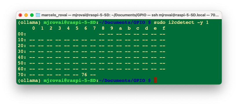
In my case, the bus address is 0x76, so we should define it in the code.
Installing the BMP 280 Library:
Once the sensor is connected, we must install its library on our Raspi. For that, we should install the Adafruit_CircuitPython_BMP280.
pip install adafruit-circuitpython-bmp280Create a new Python script as below and name it, for example, bmp280_test.py:
import time
import board

import adafruit_bmp280

i2c = board.I2C()
bmp280 = adafruit_bmp280.Adafruit_BMP280_I2C(i2c, address = 0x76)
bmp280.sea_level_pressure = 1013.25

while True:
    print("\nTemperature: %0.1f C" % bmp280.temperature)
    print("Pressure: %0.1f hPa" % bmp280.pressure)
    print("Altitude = %0.2f meters" % bmp280.altitude)
    time.sleep(2)
Execute the script:
python bmp280Test.pyThe Terminal shows the result.
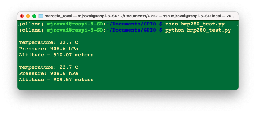
Note that pressure is presented in hPa. See the next section to better understand this unit.
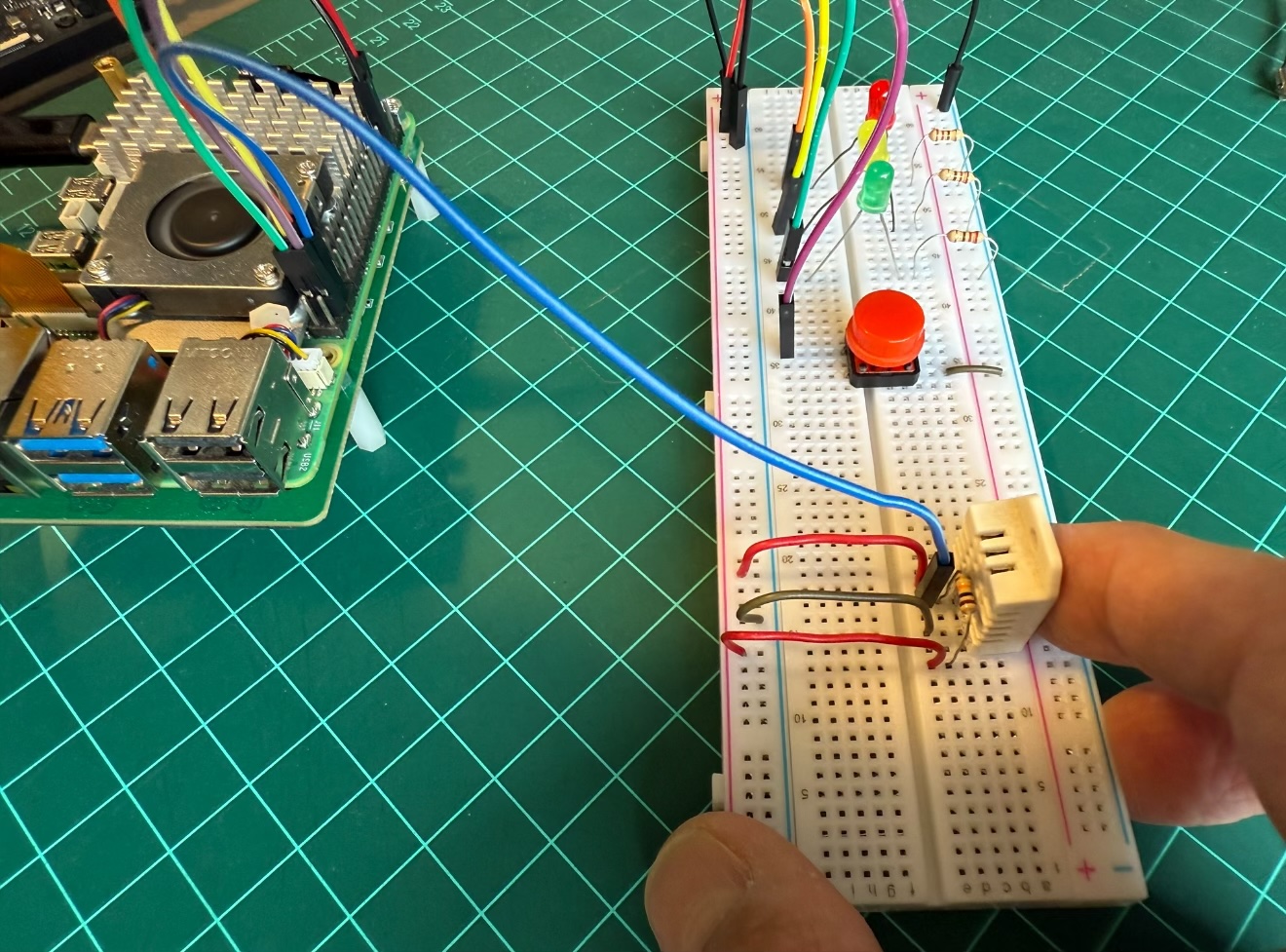
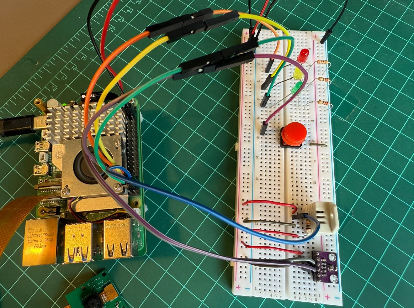
Below is the complete setup for our SLM tests.
Measuring Weather and Altitude With BMP280

Let’s take some time to understand more about what we will get with the BMP readings.
You can skip this part of the tutorial, or return later.
The BMP280 (and its predecessor, the BMP180) was designed to measure atmospheric pressure accurately. Atmospheric pressure varies with both weather and altitude.
What is Atmospheric Pressure?
Atmospheric pressure is a force that the air around you exerts on everything. The weight of the gasses in the atmosphere creates atmospheric pressure. A standard unit of pressure is “pounds per square inch” or psi. We will use the international notation, newtons per square meter, called pascals (Pa).
If you took 1 cm wide column of air would weigh about 1 kg
This weight, pressing down on the footprint of that column, creates the atmospheric pressure that we can measure with sensors like the BMP280. Because that cm-wide column of air weighs about 1 kg, the average sea level pressure is about 101,325 pascals, or better, 1013.25 hPa (1 hPa is also known as milibar - mbar). This will drop about 4% for every 300 meters you ascend. The higher you get, the less pressure you’ll see because the column to the top of the atmosphere is much shorter and weighs less. This is useful because you can determine your altitude by measuring the pressure and doing math.
The air pressure at 3,810 meters is only half that at sea level.
The BMP280 outputs absolute pressure in hPa (mbar). One pascal is a minimal amount of pressure, approximately the amount that a sheet of paper will exert resting on a table. You will often see measurements in hectopascals (1 hPa = 100 Pa). The library here provides outputs of floating-point values in hPa, equaling one millibar (mbar).
Here are some conversions to other pressure units:
- 1 hPa = 100 Pa = 1 mbar = 0.001 bar
- 1 hPa = 0.75006168 Torr
- 1 hPa = 0.01450377 psi (pounds per square inch)
- 1 hPa = 0.02953337 inHg (inches of mercury)
- 1 hPa = 0.00098692 atm (standard atmospheres)
Temperature Effects
Because temperature affects the density of a gas, density affects the mass of a gas, and mass affects the pressure (whew), atmospheric pressure will change dramatically with temperature. Pilots know this as “density altitude”, which makes it easier to take off on a cold day than a hot one because the air is denser and has a more significant aerodynamic effect. To compensate for temperature, the BMP280 includes a rather good temperature sensor and a pressure sensor.
To perform a pressure reading, you first take a temperature reading, then combine that with a raw pressure reading to come up with a final temperature-compensated pressure measurement. (The library makes all of this very easy.)
Measuring Absolute Pressure
If your application requires measuring absolute pressure, all you have to do is get a temperature reading, then perform a pressure reading (see the test script for details). The final pressure reading will be in hPa = mbar. You can convert this to a different unit using the above conversion factors.
Note that the absolute pressure of the atmosphere will vary with both your altitude and the current weather patterns, both of which are useful things to measure.
Weather Observations
The atmospheric pressure at any given location on Earth (or anywhere with an atmosphere) isn’t constant. The complex interaction between the earth’s spin, axis tilt, and many other factors result in moving areas of higher and lower pressure, which in turn cause the variations in weather we see every day. By watching for changes in pressure, you can predict short-term changes in the weather. For example, dropping pressure usually means wet weather or a storm is approaching (a low-pressure system is moving in). Rising pressure usually means clear weather is coming (a high-pressure system is moving through). But remember that atmospheric pressure also varies with altitude. The absolute pressure in my home, Lo Barnechea, in Chile (altitude 960m), will always be lower than that in San Francisco (less than 2 meters, almost sea level). If weather stations just reported their absolute pressure, it would be challenging to compare pressure measurements from one location to another (and large-scale weather predictions depend on measurements from as many stations as possible).
To solve this problem, weather stations continuously remove the effects of altitude from their reported pressure readings by mathematically adding the equivalent fixed pressure to make it appear that the reading was taken at sea level. When you do this, a higher reading in San Francisco than in Lo Barnechea will always be because of weather patterns and not because of altitude.
Sea Level Pressure Calculation
The See Level Pressure can be calculated with the formula:

Where,
po = SeaLevel Pressure
p = Atmospheric Pressure
L = Temperature Lapse Rate
h = Altitude
To = Sea Level Standard Temperature
g = Earth Surface Gravitational Acceleration
M = Molar Mass Of Dry Air
R = Universal Gas Constant
Having the absolute pressure in Pa, you check the sea level pressure using the Calculator.
Or calculating in Python, where the altitude is the real altitude in meters where the sensor is located.
presSeaLevel = pres / pow(1.0 - altitude/44330.0, 5.255) Determining Altitude
Since pressure varies with altitude, you can use a pressure sensor to measure altitude (with a few caveats). The average pressure of the atmosphere at sea level is 1013.25 hPa (or mbar). This drops off to zero as you climb towards the vacuum of space. Because the curve of this drop-off is well understood, you can compute the altitude difference between two pressure measurements (p and p0) by using a specific equation. The BMP280 gives the measured altitude using bmp280Sensor.altitude.
The above explanation was based on the BMP 180 Sparkfun tutorial.
Playing with Sensors and Actuators
In this section, using the Jupyter Notebook, we will read sensors and act on actuators directly on the Pi.
On the terminal, start the Jupyter notebook server with the command (change the IP address with the one for your Raspi):
jupyter notebook --ip=192.168.4.209 --no-browser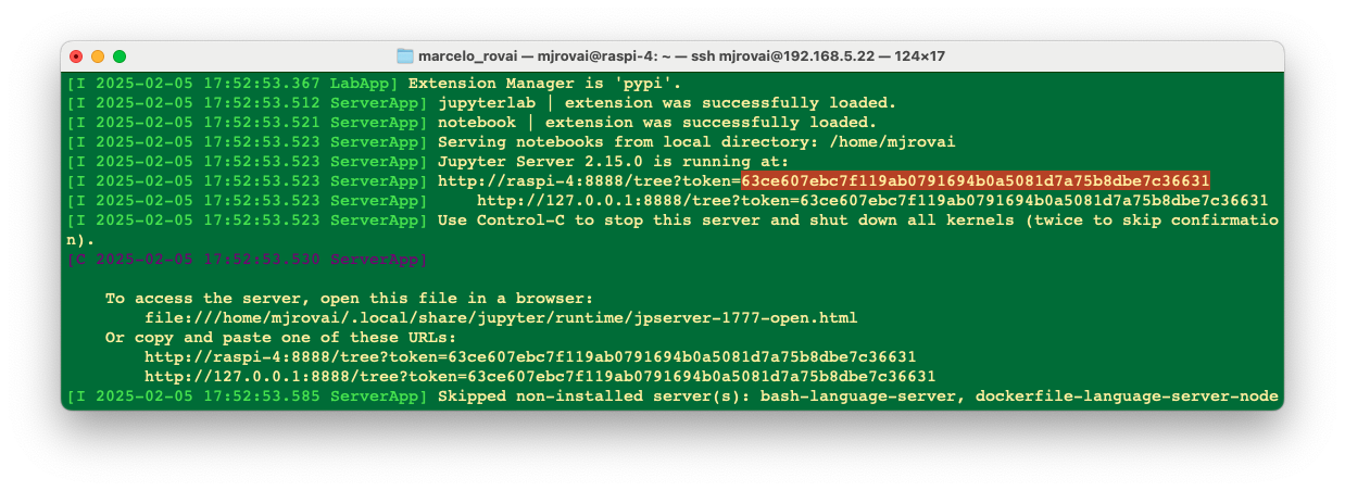
You will need the Token; you can copy it from the terminal as shown above.
The Jupyter Notebook will be running as a server on:
http:localhost:8888The first time you connect, you’ll need the token that appears in the Pi terminal when you start the notebook server.
When you start your Pi and want to use Jupyter Notebook, type the “Jupyter Notebook” command on your terminal and keep it running. This is very important! If you need to use the terminal for another task, such as running a program, open a new Terminal window.
To stop the server and close the “kernels” (the Jupyter notebooks), press [Ctrl] + [C].
Testing the Notebook setup
Let’s create a new notebook (Kernel: Python 3). Open dht_test.py, copy the code, and paste it into the notebook. That’s it. We can see the temperature and humidity values appearing on the cell. To interrupt the execution, go to the [stop] button at the top menu.
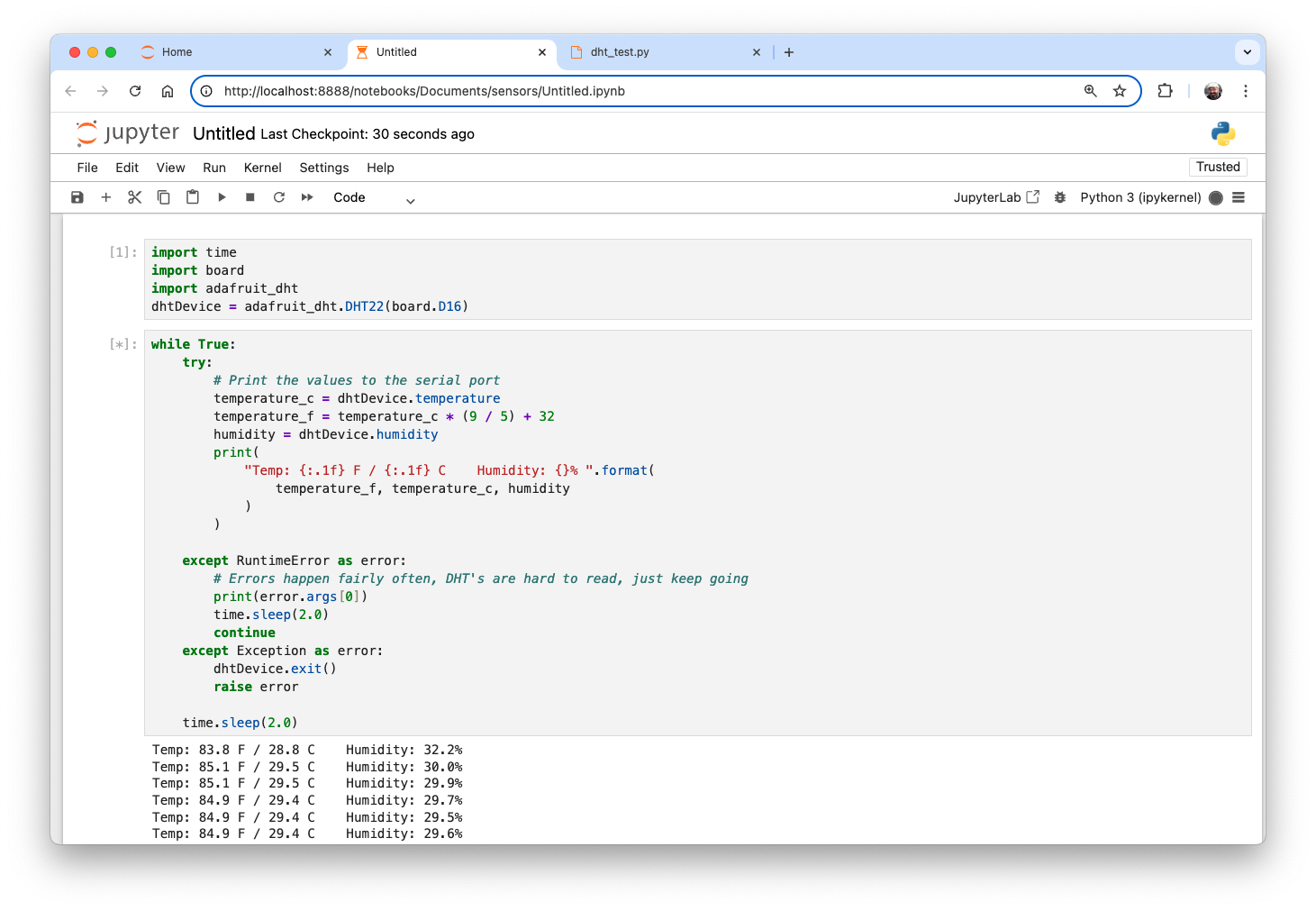
OK, this means we can access the physical world from our notebook! Let’s create a more structured code for dealing with sensors and actuators.
Initialization
Import libraries, instantiate and initialize sensors/actuators
# time library
import time
import datetime

# Adafruit DHT library (Temperature/Humidity)
import board
import adafruit_dht
DHT22Sensor = adafruit_dht.DHT22(board.D16)

# BMP library (Pressure/Temperature)
import adafruit_bmp280
i2c = board.I2C()
bmp280Sensor = adafruit_bmp280.Adafruit_BMP280_I2C(i2c, address = 0x76)
bmp280Sensor.sea_level_pressure = 1013.25

# LEDs
from gpiozero import LED

ledRed = LED(13)
ledYlw = LED(19)
ledGrn = LED(26)

ledRed.off()
ledYlw.off()
ledGrn.off()

# Push-Button
from gpiozero import Button
button = Button(20)
GPIO Input and Output
Create a function to get GPIO status:
# Get GPIO status data
def getGpioStatus():
    global timeString
    global buttonSts
    global ledRedSts
    global ledYlwSts
    global ledGrnSts

    # Get time of reading
    now = datetime.datetime.now()
    timeString = now.strftime("%Y-%m-%d %H:%M")

    # Read GPIO Status
    buttonSts = button.is_pressed
    ledRedSts = ledRed.is_lit
    ledYlwSts = ledYlw.is_lit
    ledGrnSts = ledGrn.is_lit
And another to print the status:
# Print GPIO status data
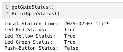
def PrintGpioStatus():
print ("Local Station Time: ", timeString)
print ("Led Red Status: ", ledRedSts)
print ("Led Yellow Status: ", ledYlwSts)
print ("Led Green Status: ", ledGrnSts)
print ("Push-Button Status: ", buttonSts)Now, we can, for example, turn on the LEDs:
ledRed.on()
ledYlw.on()
ledGrn.on()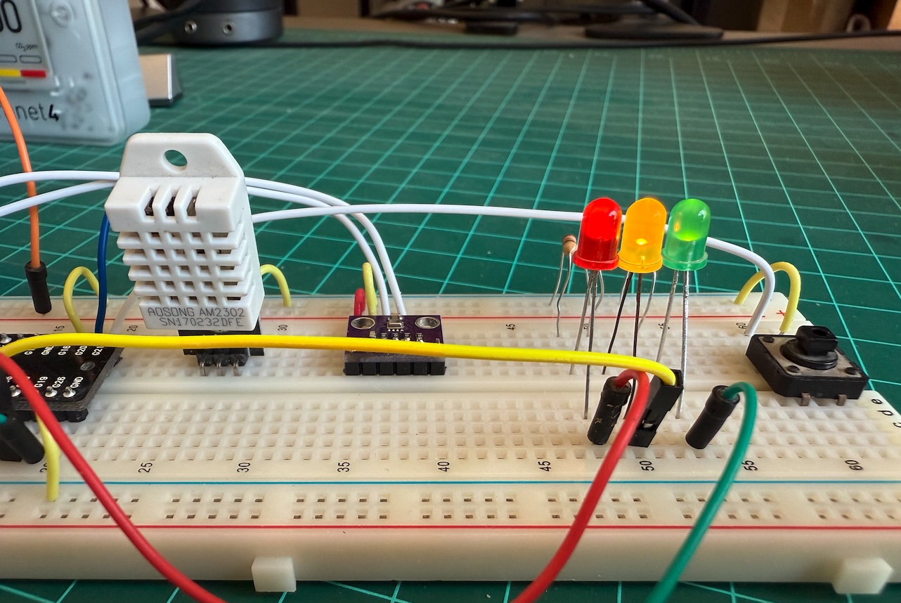
And see their status:
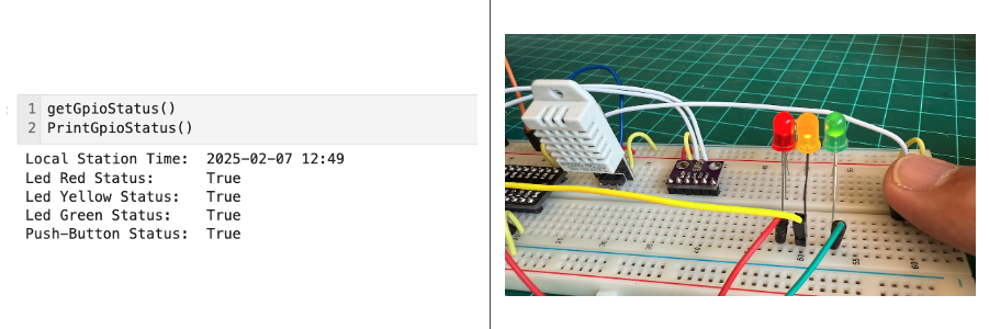
If you press the push-button, its status will also be shown:
And turning off the LEDS:
ledRed.off()
ledYlw.off()
ledGrn.off()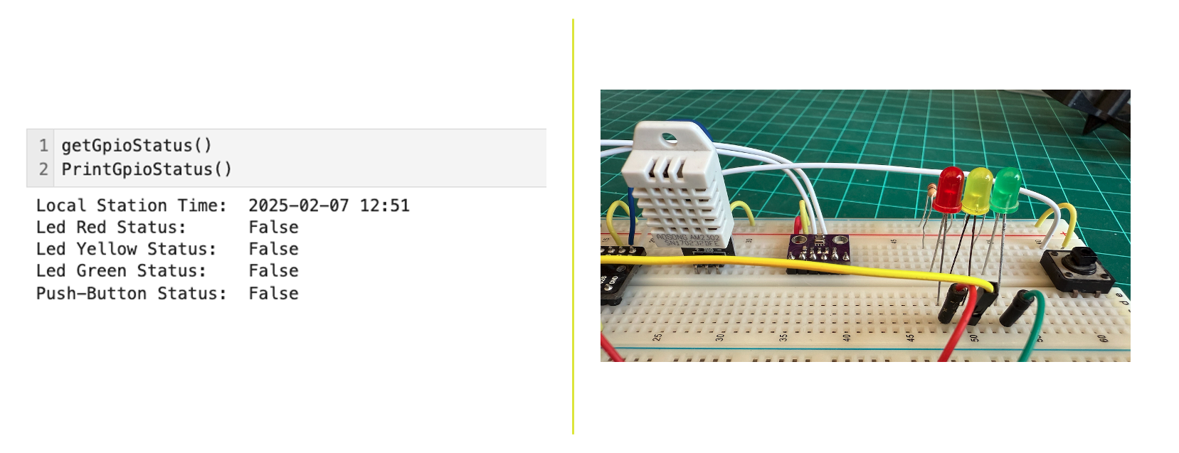
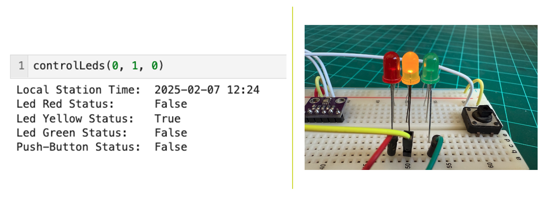
We can create a function to simplify turning LEDs on and off:
# Acting on GPIOs and printing Status
def controlLeds(r, y, g):
    if (r):
        ledRed.on()
    else:
        ledRed.off()
    if (y):
        ledYlw.on()
    else:
        ledYlw.off()
    if (g):
        ledGrn.on()
    else:
        ledGrn.off()

    getGpioStatus()
    PrintGpioStatus()
For example, turning on the Yellow LED:
Getting and displaying Sensor Data
First, we should create a function to read the BMP280 and calculate the pressure value at sea level, once the sensor only gives us the absolute pressure based on the actual altitude:
# Read data from BMP280
def bmp280GetData(real_altitude):

    temp = bmp280Sensor.temperature
    pres = bmp280Sensor.pressure
    alt =  bmp280Sensor.altitude
    presSeaLevel = pres / pow(1.0 - real_altitude/44330.0, 5.255)

    temp = round (temp, 1)
    pres = round (pres, 2) # absolute pressure in mbar
    alt = round (alt)
    presSeaLevel = round (presSeaLevel, 2) # absolute pressure in mbar

    return temp, pres, alt, presSeaLevel
Entering the BMP280 real altitude where it is located, run the code:
bmp280GetData(960)As a result, we will get (26.9, 906.73, 927, 1017.29)which means:
- Temperature of 26.9 oC
- Absolute Pressure of 906.73 hPa
- Measured Altitude (from Pressure) of 927 m
- Sea Level converted Pressure: 1,017.29 hPa
Now, we will generate a unique function to get the BMP280 and the DHT data, including a timestamp:
# Get data (from local sensors)
def getSensorData(altReal=0):
    global timeString
    global humExt
    global tempLab
    global tempExt
    global presSL
    global altLab
    global presAbs
    global buttonSts

    # Get time of reading
    now = datetime.datetime.now()
    timeString = now.strftime("%Y-%m-%d %H:%M")

    tempLab, presAbs, altLab, presSL = bmp280GetData(altReal)

    tempDHT =  DHT22Sensor.temperature
    humDHT =  DHT22Sensor.humidity

    if humDHT is not None and tempDHT is not None:
        tempExt = round (tempDHT)
        humExt = round (humDHT)
And another function to print the values:
# Display important data on-screen
def printData():
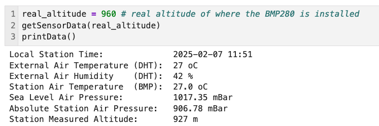
print ("Local Station Time: ", timeString)
print ("External Air Temperature (DHT): ", tempExt, "oC")
print ("External Air Humidity (DHT): ", humExt, "%")
print ("Station Air Temperature (BMP): ", tempLab, "oC")
print ("Sea Level Air Pressure: ", presSL, "mBar")
print ("Absolute Station Air Pressure: ", presAbs, "mBar")
print ("Station Measured Altitude: ", altLab, "m")Runing them:
real_altitude = 960 # real altitude of where the BMP280 is installed
getSensorData(real_altitude)
printData()
Results:
Using Python, we can command the actuators (LEDs) and read the sensors and GIPOs status at this stage. This is important, for example, to generate a data log to be read by an SLM in the future.
The notebook can be found on Github: Monitoring_Actuating_GPIOs.ipynb
⚠️ IMPORTANT: The Notebook Kernel should end after using to liberate GPIOs
The problem is that Jupyter Notebook is still holding onto the GPIO pins even after our code finishes running. When we try to run it from the terminal, those pins are already claimed by the Jupyter process. So, before running a code that deals with GPIO in the terminal, In Jupyter:
Click Kernel → Restart Kernel
Or: Click Kernel → Shutdown Kernel
Widgets
pywidgets, or jupyter-widgets orwidgets, are interactive HTML widgets for Jupyter notebooks and the IPython kernel. Notebooks come alive when interactive widgets are used. We can gain control of our data and visualize changes in them.
Widgets are eventful Python objects that have a representation in the browser, often as a control like a slider, text box, etc. We can use widgets to build interactive GUIs for our project.
In this lab, for example, we will use a slide bar to control the state of actuators in real time, such as by turning on or off the LEDs. Widgets are great for adding more dynamic behavior to Jupyter Notebooks.
Installation
To use Widgets, we must install the Ipywidgets library using the commands:
pip install ipywidgetsAfter installation, we should call the library:
# widget library
from ipywidgets import interactive
import ipywidgets as widgetsfrom
IPython.display import display
And running the below line, we can control the LEDs in real-time:
f = interactive(controlLeds, r=(0,1,1), y=(0,1,1), g=(0,1,1))
display(f)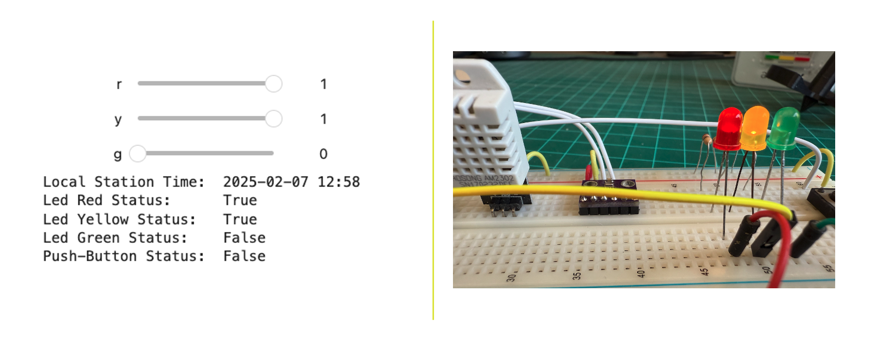
This interactive widget is very easy to implement and very powerful. You can learn more about Interactive on this link: Interactive Widget.
Advanced GPIO Zero Features
GPIO Zero includes many advanced features that make complex projects much easier to build.
PWM LED Brightness Control
Use PWMLED to control LED brightness:
from gpiozero import PWMLED
from time import sleep

led = PWMLED(13)

# Fade in and out
while True:
    led.pulse() # Smooth fade in and out
  sleep(5)
Composite Devices
Create a traffic light system with one object:
from gpiozero import TrafficLights
from time import sleep

lights = TrafficLights(red=13, amber=19, green=26)

while True:
  lights.red.on()
  sleep(2)
  lights.amber.on()
  sleep(1)
  lights.red.off()
  lights.amber.off()
  lights.green.on()
  sleep(3)
  lights.green.off()
  lights.amber.on()
  sleep(1)
  lights.amber.off()
Other Useful GPIO Zero Devices
Buzzer:
from gpiozero import BuzzerMotor:
from gpiozero import MotorServo:
from gpiozero import ServoDistanceSensor:
from gpiozero import DistanceSensorMotionSensor:
from gpiozero import MotionSensorRobot:
from gpiozero import Robot
Interacting an SLM with the Physical world
This section demonstrates in a simple way how to integrate a Small Language Model (SLM) with the sensors and LEDs we have set up. The diagram below shows how data flows from sensors through processing and AI analysis to control the actuators and ultimately provide user feedback.
We will use the Transformers library from Hugging Face for model loading and inference. This library provides the architecture for working with pre-trained language models, helping interact with the model, processing input prompts, and obtaining outputs.
Installation
pip install transformers torchLet’s create a simple SLM test in the Jupyter Notebook that checks if the model loads and measures inference time. The model used here is the TinyLLama 1.1B. We will ask a straightforward question:
"The weather today is"As a result, besides the SLM answer, we will also measure the latency.
Run this script:
import time
from transformers import pipeline
import torch
# Check if CUDA is available (it won't be on our case, Raspberry Pi)
device = "cuda" if torch.cuda.is_available() else "cpu"
print(f"Using device: {device}")
# Load the model and measure loading time
start_time = time.time()
model='TinyLlama/TinyLlama-1.1B-intermediate-step-1431k-3T'
generator = pipeline('text-generation',
model=model,
device=device)
load_time = time.time() - start_time
print(f"Model loading time: {load_time:.2f} seconds")
# Test prompt
test_prompt = "The weather today is"
# Measure inference time
start_time = time.time()
response = generator(test_prompt,
max_length=50,
num_return_sequences=1,
temperature=0.7)
inference_time = time.time() - start_time
print(f"\nTest prompt: {test_prompt}")
print(f"Generated response: {response[0]['generated_text']}")
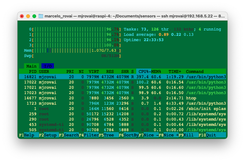
print(f"Inference time: {inference_time:.2f} seconds")As we can see, the SLM works, but the latency is very high (+3 minutes). It is OK because this particular test is on a Raspberry Pi 4. With a Raspberry Pi 5, the result would be better.:
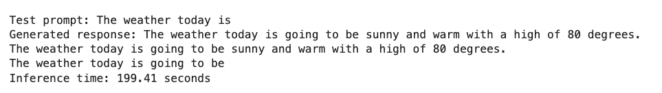
The Raspi uses around 1GB of memory (model + process) and all four cores to process the answer. The model alone needs around 800MB.
Now, let us create a code showing a basic interaction pattern where the SLM can respond to sensor data and interact with the LEDs.
Install the Libraries:
import time
import datetime
import board
import adafruit_dht
import adafruit_bmp280
from gpiozero import LED, Button
from transformers import pipeline
Initialize sensors
DHT22Sensor = adafruit_dht.DHT22(board.D16)
i2c = board.I2C()
bmp280Sensor = adafruit_bmp280.Adafruit_BMP280_I2C(i2c, address=0x76)
bmp280Sensor.sea_level_pressure = 1013.25
Initialize LEDs and Button
ledRed = LED(13)
ledYlw = LED(19)
ledGrn = LED(26)
button = Button(20)
Initialize the SLM pipeline
# We're using a small model suitable for Raspberry Pi

model='TinyLlama/TinyLlama-1.1B-intermediate-step-1431k-3T'
generator = pipeline('text-generation',
                    model=model,
                    device='cpu')
Support Functions
Now, let’s create support functions for readings from all sensors and control the LEDs:
def get_sensor_data():
    """Get current readings from all sensors"""
    try:
        temp_dht = DHT22Sensor.temperature
        humidity = DHT22Sensor.humidity
        temp_bmp = bmp280Sensor.temperature
        pressure = bmp280Sensor.pressure

        return {
            'temperature_dht': round(temp_dht, 1) if temp_dht else None,
            'humidity': round(humidity, 1) if humidity else None,
            'temperature_bmp': round(temp_bmp, 1),
            'pressure': round(pressure, 1)
        }
    except RuntimeError:
        return None


def control_leds(red=False, yellow=False, green=False):
    """Control LED states"""
    ledRed.value = red
    ledYlw.value = yellow
    ledGrn.value = green


def process_conditions(sensor_data):
    """Process sensor data and control LEDs based on conditions"""
    if not sensor_data:
        control_leds(red=True)  # Error condition
        return

    temp = sensor_data['temperature_dht']
    humidity = sensor_data['humidity']

    # Example conditions for LED control
    if temp > 30:  # Hot
        control_leds(red=True)
    elif humidity > 70:  # Humid
        control_leds(yellow=True)
    else:  # Normal conditions
        control_leds(green=True)
Generating an SLM’s response
So far, the LEDs reaction is only based on logic, but let’s also use the SLM to “analyse” the sensors condition, generating a response based on that:
def generate_response(sensor_data):
    """Generate response based on sensor data using SLM"""
    if not sensor_data:
        return "Unable to read sensor data"

    prompt = f"""Based on these sensor readings:
    Temperature: {sensor_data['temperature_dht']}°C
    Humidity: {sensor_data['humidity']}%
    Pressure: {sensor_data['pressure']} hPa

    Provide a brief status and recommendation in 2 sentences.
    """

    # Generate response from SLM
    response = generator(prompt,
                       max_length=100,
                       num_return_sequences=1,
                       temperature=0.7)[0]['generated_text']

    return response
Main Function
And now, let’s create a main() function to wait for the user to, for example, press a button and, capture the data generated by the sensors, delivering some observation or recommendation from the SLM:
def main_loop():
    """Main program loop"""
    print("Starting Physical Computing with SLM Integration...")
    print("Press the button to get a reading and SLM response.")

    try:
        while True:
            if button.is_pressed:
                # Get sensor readings
                sensor_data = get_sensor_data()

                # Process conditions and control LEDs
                process_conditions(sensor_data)

                if sensor_data:
                    # Get SLM response
                    response = generate_response(sensor_data)

                    # Print current status
                    print("\nCurrent Readings:")
                    print(f"Temperature: {sensor_data['temperature_dht']}°C")
                    print(f"Humidity: {sensor_data['humidity']}%")
                    print(f"Pressure: {sensor_data['pressure']} hPa")
                    print("\nSLM Response:")
                    print(response)

                time.sleep(2)  # Debounce and allow time to read

            time.sleep(0.1)  # Reduce CPU usage

    except KeyboardInterrupt:
        print("\nShutting down...")
        control_leds(False, False, False)  # Turn off all LEDs
Test Result
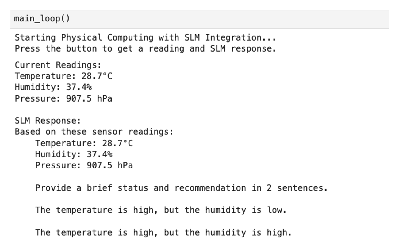
The sensors are read after the user presses the button to trigger a reading, and LEDs are controlled based on conditions. Sensor data is formatted into a prompt for the SLM to generate a response analyzing the current conditions. The results are displayed in the terminal, and the LED indicators are shown.
- Red: High temperature (>30°C) or error condition
- Yellow: High humidity (>70%)
- Green: Normal conditions
This simple code integrates a Small Language Model (TinyLlama model (1.1B parameters) with our physical computing setup, providing raw sensor data and intelligent responses from the SLM about the environmental conditions.
We can extend this first test to more sophisticated and valuable uses of the SLM integration, for example: adding:
- Starting the process from a User Prompt.
- Receive commands from the User to switch LEDs ON or OFF
- Provide the status of LEDS, Button, or specific sensor data from the user prompt
- Log data and responses to a file. Provide historical information by user request
- Implement different types of prompts for various use cases
Other Models
We can use other SLMs in a Raspberry Pi that have distinct ways of handling them. For example, many modern models use GGUF formats, and to use them, we need to install llama-cpp-python, which is designed to work with GGUF models.
Also, as we saw in a previous lab, Ollama is a great way to download and test SLMs on the Raspberry Pi.
Conclusion
Key Achievements
Throughout this tutorial, we’ve successfully: - Set up a complete physical computing environment using Raspberry Pi - Integrated multiple environmental sensors (DHT22 and BMP280) - Implemented visual feedback through LED actuators - Created interactive controls using push buttons - Integrated a Small Language Model (TinyLLama 1.1B) for intelligent analysis - Developed a foundation for AI-enhanced environmental monitoring
Technical Insights
Hardware Integration
The combination of digital (DHT22) and I2C (BMP280) sensors demonstrated different communication protocols and their implementations. This multi-sensor approach provides redundancy and comprehensive environmental monitoring capabilities. The LED actuators and push-button interface created a responsive and interactive system that bridges the digital and physical worlds.
Software Architecture
The layered software architecture we developed supports: 1. Low-level sensor communication and actuator control 2. Data preprocessing and validation 3. SLM integration for intelligent analysis 4. Interactive user interfaces through both hardware and software
AI Integration Learnings
The integration of TinyLLama 1.1B revealed several important insights: - Small Language Models can effectively run on edge devices like Raspberry Pi - Natural language processing can enhance sensor data interpretation - Real-time analysis is possible, though with some latency considerations - The system can provide human-readable insights from complex sensor data
Practical Applications
This project serves as a foundation for numerous real-world applications: - Environmental monitoring systems - Smart home automation - Industrial sensor networks - Educational platforms for IoT and AI integration - Prototyping platforms for larger-scale deployments
Challenges and Solutions
Throughout the development, we encountered and addressed several challenges: 1. Resource Constraints: - Optimized SLM inference for Raspberry Pi capabilities - Implemented efficient sensor reading strategies - Managed memory usage for stable operation
- Data Integration:
- Developed robust sensor data validation
- Created effective data preprocessing pipelines
- Implemented error handling for sensor failures
- AI Integration:
- Designed effective prompting strategies
- Managed inference latency
- Balanced accuracy with response time
Future Enhancements
The system can be extended in several directions: 1. Hardware Expansions: - Additional sensor types (air quality, light, motion) - Camera for IA applications - More complex actuators (displays, motors, relays) - Wireless connectivity options as WiFI, BLE, or LoRa 2. Software Improvements: - Advanced data logging and analysis - Web-based monitoring interface - Real-time visualization tools 3. AI Capabilities: 1. Models for detecting and counting objects 2. RAG or Fine-tuning SLM for specific applications 3. Multi-modal AI integration via sensor integration 4. Automated decision-making systems 5. Predictive maintenance capabilities
Final Thoughts
This chapter demonstrates that integrating physical computing with AI is feasible and practical on readily accessible hardware such as the Raspberry Pi. Combining sensors, actuators, and AI creates a powerful platform for developing intelligent environmental monitoring and control systems.
While the current implementation focuses on environmental monitoring, the principles and techniques can be adapted to various applications. The modular nature of hardware and software components allows for customization and expansion based on specific needs.
Integrating small language models into physical computing opens new possibilities for creating more intuitive and intelligent IoT devices. As edge AI capabilities evolve, projects like this will become increasingly important in developing the next generation of smart devices and systems.
Remember that this is just the beginning. Our foundation can be extended in countless ways to create more sophisticated and capable systems. The key is to build on these basics while balancing functionality, reliability, and resource usage.